Start with a two-matrix probability law
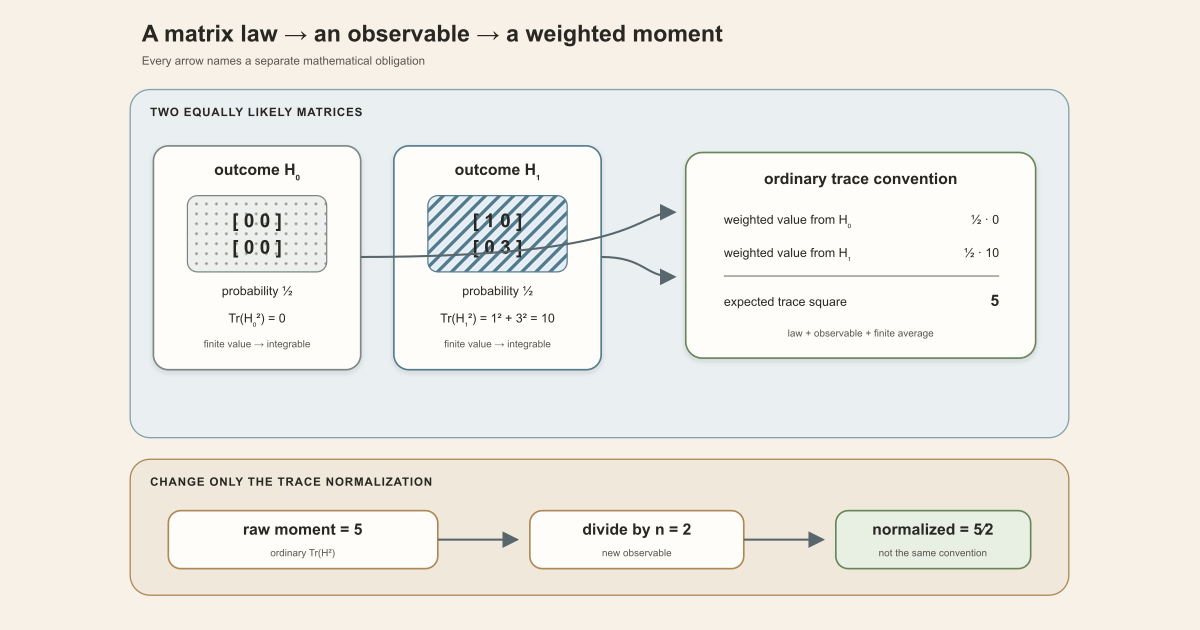
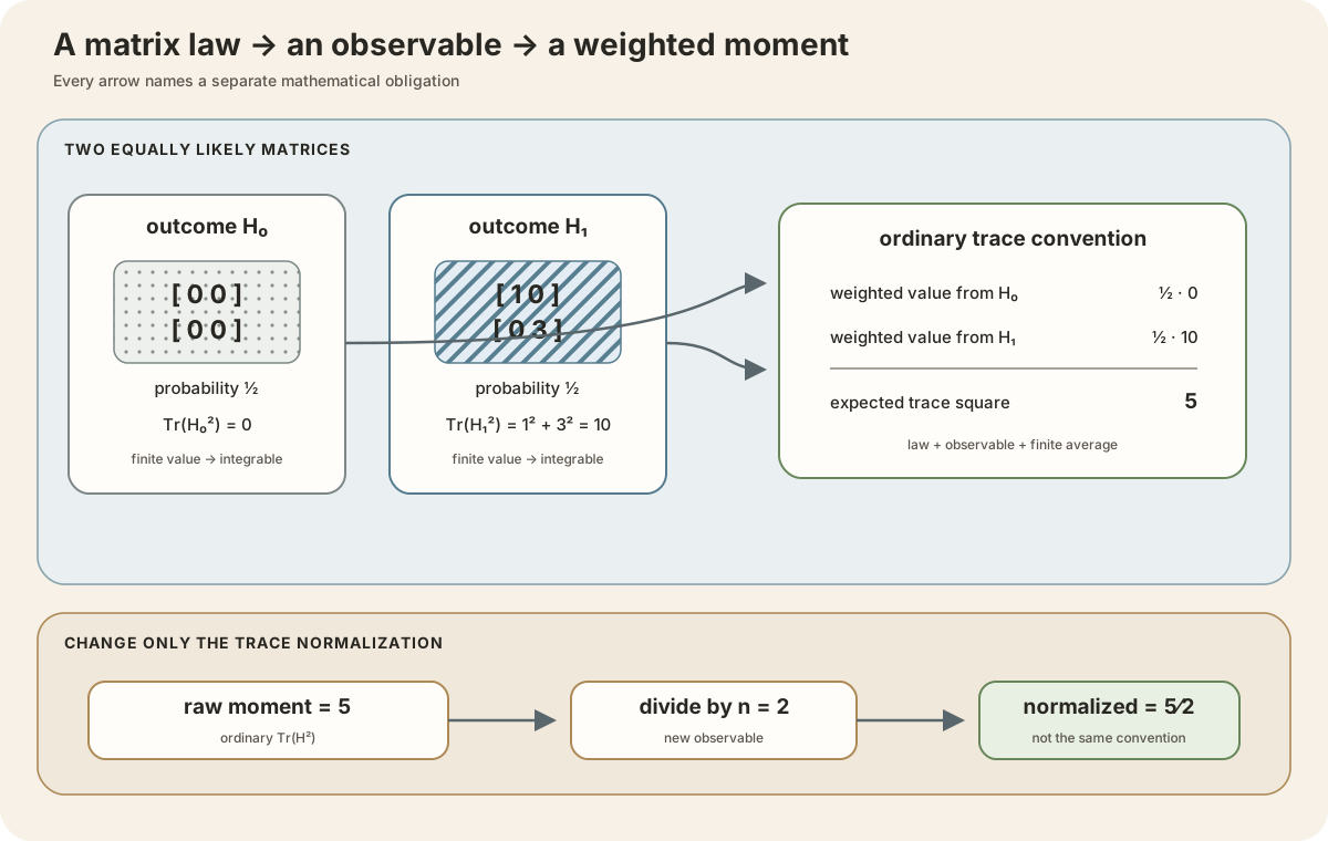
Before introducing Gaussian coordinates, put equal probability on two deterministic Hermitian matrices:
\[ H_0= \begin{pmatrix} 0&0\\ 0&0 \end{pmatrix}, \qquad H_1= \begin{pmatrix} 1&0\\ 0&3 \end{pmatrix}, \qquad \mathbb P(H=H_0)=\mathbb P(H=H_1)=\frac12. \]For the second trace power,
\[ \operatorname{Tr}(H_0^2)=0, \qquad \operatorname{Tr}(H_1^2)=1^2+3^2=10. \]The finite trace moment is therefore
\[ \mathbb E[\operatorname{Tr}(H^2)] =\frac12\cdot0+\frac12\cdot10 =5. \]Everything is visible in this finite model. The law supplies the two weights, the observable turns each matrix into one number, integrability is automatic because only two finite values occur, and expectation performs the weighted average. If we instead use normalized trace for these two-by-two matrices, the answer is
\[ \mathbb E\!\left[\frac12\operatorname{Tr}(H^2)\right] =\frac52. \]That factor of two is a convention change, not an algebra mistake.
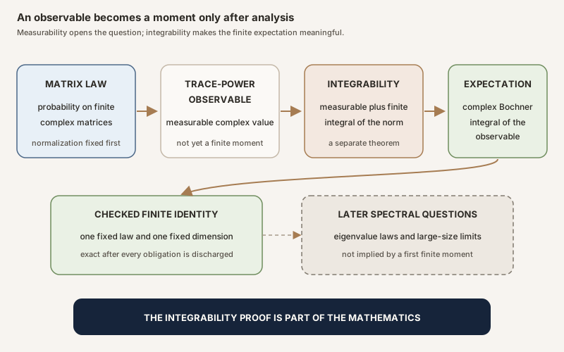
A finite matrix trace moment is the expected value of the trace of a fixed power of a finite random matrix. Three words in that sentence carry separate obligations: the matrix has a specified probability law, the trace power is a measurable complex-valued observable, and the observable is integrable.
Let \(\mu\) be a probability measure on complex \(n\)-by-\(n\) matrices, and let \(k\) be a nonnegative integer. When the function \(H\mapsto\operatorname{Tr}(H^k)\) is integrable under \(\mu\), its trace moment is
\[ m_k(\mu) =\int \operatorname{Tr}(H^k)\,\mathrm d\mu(H). \]The project uses the ordinary, unnormalized matrix trace. A normalized-trace moment would instead divide by the matrix dimension and is a different quantity. Neither convention should be inferred from the word moment alone. The complex Bochner integral in the definition is the norm-controlled integral for complex-valued functions; its integrability gate is explained below.
Observable, integrability, and moment are different layers
\[ T_k(H)=\operatorname{Tr}(H^k) \]is defined pointwise. Measurability says that inverse images of measurable sets are measurable, so \(T_k\) is eligible to participate in measure theory. It does not bound the size of \(T_k\).
For a complex-valued function, Bochner integrability requires strong measurability up to a null set and finite integral of the complex norm (Mathlib contributors):
\[ \int \lVert T_k(H)\rVert\,\mathrm d\mu(H)\lt\infty. \]Only after this analytic condition is available does the displayed complex
integral behave as the expected trace power. This separation matters especially
in Lean. Mathlib’s Bochner integral is a total function: outside the integrable
case its definition returns zero. Therefore an isolated equation involving an
integral could conceal a failed integrability obligation. The project pairs
each exact identity with an explicit Integrable theorem.
The codomain is ℂ because the ambient matrix space is complex. If the law is concentrated on Hermitian matrices, then every trace power is real-valued almost everywhere under that law, but the integral is still stated in the ambient complex codomain. Reality and integrability remain distinct facts.
Why a probability measure turns the integral into expectation
An expectation is an integral with respect to a probability measure. The
project’s finite Gaussian unitary ensemble (GUE) matrix law already has an
IsProbabilityMeasure instance, so no additional normalization by
the total mass is needed:
For a general finite measure, the same integral need not equal an average unless one divides by the total mass. Calling every finite-measure integral an expectation would silently change the convention.
Pushforward laws let the integral move to useful coordinates
Suppose a measurable map \(F:X\to Y\) transports a source measure \(\nu\) to \(\mu\), so \(\mu\) is the pushforward \(F_*\nu\). Under the corresponding measurability and integrability hypotheses,
\[ \int_Y g(y)\,\mathrm d(F_*\nu)(y) =\int_X g(F(x))\,\mathrm d\nu(x). \]This is not only a computational convenience. It preserves the exact law while moving the observable to a space where its algebra is transparent. For finite GUE, the ambient matrix law is represented as the pushforward of a normalized real Hermitian coordinate law. Composing the observable with that assembly map moves the integral to the coordinate space. The first two trace powers then reduce to finite sums of ordinary real Gaussian coordinates or their squares (Mathlib contributors).
Integrability must move through the pushforward too. One proves the composed source observable integrable and transfers that fact to the target law, or uses the appropriate equivalence supplied by the measurable map. The integral identity does not erase that obligation.
The first power reads only the diagonal
For every finite square matrix,
\[ \operatorname{Tr}(H)=\sum_{i=0}^{n-1}H_{ii}. \]Under the project’s centered finite GUE law, each complex-valued diagonal coordinate has a centered Cartesian complex Gaussian law with real-coordinate variance \(s_n\) and imaginary-coordinate variance zero, where \(s_0=0\) and \(s_n=1/n\) for positive dimension. It is therefore real almost surely. Each coordinate is integrable and has complex mean zero (Mathlib contributors). Finite linearity of the Bochner integral therefore gives
\[ \mathbb E[\operatorname{Tr}(H)]=0. \]Off-diagonal entries do not enter this calculation. Neither independence nor unitary invariance is needed for the first identity once the centered diagonal marginals are known.
The second power includes every Hermitian entry
For a Hermitian matrix, conjugate symmetry turns the trace square into the Frobenius norm square:
\[ \begin{aligned} \operatorname{Tr}(H^2) &=\sum_{i,j}H_{ij}H_{ji}\\ &=\sum_{i,j}H_{ij}\overline{H_{ij}}\\ &=\sum_{i,j}|H_{ij}|^2 =\lVert H\rVert_F^2. \end{aligned} \]Now write \(H\) in normalized Hermitian coordinates . There is one real orthonormal coordinate for every ambient matrix position, so the coordinate index has cardinality \(n^2\). If those real coordinates are \(z_a\), then
\[ \operatorname{Tr}(H^2)=\sum_a z_a^2. \]Every \(z_a\) is centered Gaussian with variance \(s_n\). Hence finite linearity and the scalar second-moment formula yield
\[ \mathbb E[\operatorname{Tr}(H^2)] =n^2s_n =n \]for positive \(n\). At \(n=0\), the coordinate index is empty, the matrix is the unique empty matrix, and both sides are zero. The formal theorem handles both branches.
Independence is not used in the final sum. Expectation is linear even for dependent summands. The product-law construction is still important because it established the exact normalized coordinate law and its scalar marginals, but no cross term appears in the norm-square expression.
Normalization ledger for the checked finite GUE moments
| Item | Project convention | Consequence here |
|---|---|---|
| Dimension | \(n\in\mathbb N\), including zero | Theorems require no positivity hypothesis |
| Diagonal variance | \(1/n\) for positive \(n\) | Each diagonal contributes \(1/n\) to the second moment |
| Off-diagonal displayed variances | Real and imaginary parts each have variance \(1/(2n)\) | Their two reflected matrix entries have the correct total Frobenius weight |
| Normalized real coordinates | Diagonal, scaled upper-real, and scaled upper-imaginary coordinates each have variance \(1/n\) | One homogeneous real Gaussian product |
| Coordinate count | \(n^2\) | The expected squared Frobenius norm is \(n^2/n=n\) |
| Trace | Ordinary, unnormalized trace | The second expected trace power is \(n\), not \(1\) |
| Zero dimension | Variance scale zero and empty coordinate family | Both checked moments are zero |
| Density and eigenvalues | Not used | No Jacobian, spectral theorem, or eigenvalue enumeration enters the proof |
The often-quoted positive-dimensional identity \(\mathbb E[n^{-1}\operatorname{Tr}(H^2)]=1\) follows on paper by dividing the checked second identity by \(n\). That normalized statement is not the theorem formalized here, and it has no literal \(n=0\) form without an additional convention.
In Lean
GUE.integral_tracePower_two nGUEis the project namespace for the chosen finite Gaussian unitary ensemble convention.integral_tracePower_twonames the theorem; the wordintegralkeeps the operation explicit, whiletracePower_twofixes both observable and exponent.n : ℕis the matrix dimension. The theorem deliberately includesn = 0.- The full elaborated conclusion below contains
∂GUE.matrixLaw n, so the measure is not inferred from prose. - The right side is coerced to
ℂbecause the trace-power observable and Bochner integral are complex-valued. - This theorem uses the ordinary trace. It does not hide the divisor \(1/n\).
The RMT-09 module states four theorems for every natural dimension:
theorem GUE.integrable_tracePower_one (n : ℕ) :
    MeasureTheory.Integrable
      (RandomMatrix.tracePower
        (id : Matrix (Fin n) (Fin n) ℂ → Matrix (Fin n) (Fin n) ℂ) 1)
      (GUE.matrixLaw n)

theorem GUE.integral_tracePower_one (n : ℕ) :
    ∫ H : Matrix (Fin n) (Fin n) ℂ,
        RandomMatrix.tracePower id 1 H ∂GUE.matrixLaw n = 0

theorem GUE.integrable_tracePower_two (n : ℕ) :
    MeasureTheory.Integrable
      (RandomMatrix.tracePower
        (id : Matrix (Fin n) (Fin n) ℂ → Matrix (Fin n) (Fin n) ℂ) 2)
      (GUE.matrixLaw n)

theorem GUE.integral_tracePower_two (n : ℕ) :
    ∫ H : Matrix (Fin n) (Fin n) ℂ,
        RandomMatrix.tracePower id 2 H ∂GUE.matrixLaw n = (n : ℂ)
Here id is the identity random matrix on the ambient matrix sample
space. It makes tracePower id k the observable
\(H\mapsto\operatorname{Tr}(H^k)\). The first and third declarations are not auxiliary
noise: they are the analytic licenses for reading the following integral
identities as finite expectations.
Type the two-point calculation locally
The following worksheet imports only Std and checks the finite law
from the opening example with exact rational arithmetic. Save it as
TwoPointTraceMoment.lean:
import Std

structure Diagonal2 where
  d0 : Int
  d1 : Int
deriving Repr

def traceSquare (H : Diagonal2) : Int :=
  H.d0 * H.d0 + H.d1 * H.d1

def H0 : Diagonal2 := { d0 := 0, d1 := 0 }
def H1 : Diagonal2 := { d0 := 1, d1 := 3 }

def rawSecondMoment : Rat :=
  (1 : Rat) / 2 * traceSquare H0 +
  (1 : Rat) / 2 * traceSquare H1

def normalizedSecondMoment : Rat :=
  rawSecondMoment / 2

#eval traceSquare H0
#eval traceSquare H1
#eval rawSecondMoment
#eval normalizedSecondMoment

example : rawSecondMoment = 5 := by native_decide
example : normalizedSecondMoment = (5 : Rat) / 2 := by native_decide
Run it on a Mac or Linux machine with the pinned toolchain already installed:
elan run leanprover/lean4:v4.32.0 lean TwoPointTraceMoment.lean
This exact worksheet was executed successfully with Lean 4.32.0 and printed:
0
10
5
(5 : Rat)/2
Both exact equality examples elaborated without error. This worksheet formalizes a finite arithmetic model, not the continuous GUE law.
The authoritative source is
formalization/NonlinearDynamics/Random/RandomMatrices/GaussianUnitaryEnsembleMoments.lean.
In a clone with the repository’s pinned Lean and Mathlib dependencies
installed, a human can make a scratch file containing:
import NonlinearDynamics.Random.RandomMatrices.GaussianUnitaryEnsembleMoments

#check NonlinearDynamics.Random.GUE.integrable_tracePower_one
#check NonlinearDynamics.Random.GUE.integral_tracePower_one
#check NonlinearDynamics.Random.GUE.integrable_tracePower_two
#check NonlinearDynamics.Random.GUE.integral_tracePower_two
The first and third checks expose the integrability licenses. The second and fourth expose the corresponding exact integral identities. The full-project command below checks the full pinned module and its Mathlib dependencies.
cd formalization
lake env lean -DwarningAsError=true NonlinearDynamics/Random/RandomMatrices/GaussianUnitaryEnsembleMoments.lean
Resource note: this exact file uses the repository's
pinned Lean and Mathlib dependencies. Initial project setup can require
substantial disk space and build time. For a lightweight first step on
macOS or Linux, use the page's standalone Lean-core or Std
tutorial.
What these moments do not establish
The checked identities do not by themselves define measurable eigenvalues, construct an empirical spectral measure, prove a joint eigenvalue density, or establish the semicircle law. They do not give higher trace moments, variances of trace powers, concentration, local spacing statistics, or universality.
The identity for the second power is consistent with an order-one spectral scale under Wigner normalization (Anderson, Guionnet, and Zeitouni; Tao). That is explanatory context, not a checked large-dimension theorem. A finite expectation at each \(n\) does not imply a limit as \(n\to\infty\). Wigner’s early large-matrix work supplies historical context for the trace-moment program, not a premise of this exact proof (Wigner).
Exercises
- For a deterministic two-by-two Hermitian matrix, expand \(\operatorname{Tr}(H^2)\) entry by entry and verify that it equals the Frobenius norm square.
- Replace the ordinary trace by \(n^{-1}\operatorname{Tr}\) for positive \(n\). Derive the corresponding first two expected values, and identify exactly where the positivity assumption is used.
- Explain why the second-moment sum needs scalar second moments but not independence between distinct coordinates.
- Construct a measurable but nonintegrable real random variable. Use it to explain why measurability alone cannot license the word expectation.
- Starting from a pushforward law \(F_*\nu\), list the separate hypotheses needed to transfer both integrability and an integral identity.
Where to continue
First Exact Finite Gaussian Unitary Ensemble Trace Moments derives both identities with every algebraic step explicit and maps them to the checked Lean proofs. The matrix trace entry fixes the algebraic operation, while Hermitian Frobenius geometry explains the norm identity behind the second moment.
For the law being integrated, read the Gaussian unitary ensemble entry and From Normalized Hermitian Coordinates to Gaussian Unitary Ensemble Invariance.
The next algebraic layer is now available in the empirical spectral measure entry and Finite Hermitian Spectra and Empirical Measures. It converts the first two trace powers into moments of a finite spectral counting measure while keeping the unresolved eigenvalue-measurability premise explicit.
References
Mathlib contributors. Bochner integral, pushforward of a measure, and matrix trace, Mathlib 4 documentation. These official APIs define the complex-valued Bochner integral, transport integration through measurable maps, and provide the finite trace algebra used here.
Mathlib contributors. Real Gaussian distributions and multivariate Gaussian distributions, Mathlib 4 documentation. These official pages document the centered scalar Gaussian moments and the finite-dimensional standard Gaussian representation.
Greg W. Anderson, Alice Guionnet, and Ofer Zeitouni. An Introduction to Random Matrices, Cambridge University Press, 2010. Chapters 2 and 3 provide the standard Wigner-matrix and Gaussian-ensemble context. Normalizations vary across the literature, so the project ledger above remains authoritative for the checked identities.
Terence Tao. Topics in Random Matrix Theory, American Mathematical Society, 2012. The trace-moment method and its spectral interpretation are developed in a standard asymptotic setting; those later results are not inferred here from the first two finite identities.
Eugene P. Wigner. Characteristic Vectors of Bordered Matrices With Infinite Dimensions, Annals of Mathematics 62 (1955), 548-564. This primary source is historical context for the large-matrix moment program, not a source for the project-specific Lean proof.
The exact upstream Lean source audited for this entry is Mathlib commit
81a5d257,
the revision pinned by formalization/lake-manifest.json.