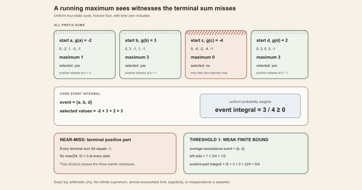
Take four equally likely states \(a,b,c,d\), let \(T\) cycle through them, and read the observable
\[ g(a)=-2,\qquad g(b)=3,\qquad g(c)=-4,\qquad g(d)=2. \]The uniform probability measure gives each state mass \(1/4\), and the cycle preserves it. Through horizon \(N=4\), include the empty sum \(S_0=0\):
| start | \(S_0,S_1,S_2,S_3,S_4\) | maximum \(M_4\) | in \(E_4=\{M_4\gt0\}\)? |
|---|---|---|---|
| \(a\) | \(0,-2,1,-3,-1\) | \(1\) | yes |
| \(b\) | \(0,3,-1,1,-1\) | \(3\) | yes |
| \(c\) | \(0,-4,-2,-4,-1\) | \(0\) | no |
| \(d\) | \(0,2,0,3,-1\) | \(3\) | yes |
Thus \(E_4=\{a,b,d\}\), and the core inequality is visible numerically:
\[ \int_{E_4}g\,d\mu =\frac{-2+3+2}{4} =\frac34\geq0. \]Individual selected points need not have positive \(g\): state \(a\) is selected even though \(g(a)=-2\).
For the strict average threshold \(1\), only \(b\) and \(d\) have some average above \(1\). Hence the event has measure \(2/4\), while
\[ 1\cdot\frac24 \leq\frac{0+3+0+2}{4} =\int_\Omega \max(g,0)\,d\mu =\frac54. \]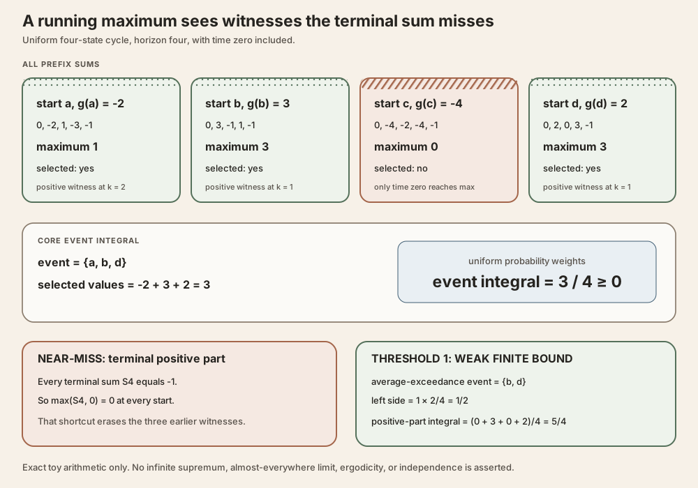
A finite maximal ergodic inequality controls, for an integrable observable under a measure-preserving transformation, the set of starting points at which at least one finite orbit sum becomes strictly positive. Its most compact form says that the original observable has nonnegative integral over that set. The theorem is finite: it takes a fixed horizon, uses a maximum over finitely many sums, and makes no assertion that orbit averages converge.
Random-matrix-theory milestone 23 (RMT-23) formalizes this result for a general measure-preserving transformation. The proof needs an integrable real observable, but it needs neither probability normalization nor ergodicity. It also does not need the transformation to be injective, surjective, or invertible.
The finite sums are the objects developed in the Birkhoff sum entry. The complete proof, historical comparison, declaration ledger, and exercises are in Finite Maximal Ergodic Inequalities: From Orbit Maxima to Threshold Events. The checked implementation narrative is The Finite Hopf Maximal Ergodic Lemma in Lean.
Exact finite objects
Let \(\Omega\) be a measurable state space, let \(\mu\) be a measure on it, let \(T:\Omega\to\Omega\) be a discrete-time transformation, and let \(g:\Omega\to\mathbb R\) be a real observable. For a starting point \(\omega\in\Omega\), define the finite Birkhoff sum
\[ S_k g(\omega) {} = \sum_{\substack{j\in\mathbb N\\j\lt k}} g\bigl(T^j\omega\bigr). \]Thus \(S_0g(\omega)=0\), \(S_1g(\omega)=g(\omega)\), and
\[ S_{j+1}g(\omega) {} = g(\omega)+S_jg(T\omega). \]Fix a finite horizon \(N\in\mathbb N\). The finite running maximum is
\[ M_Ng(\omega) {} = \max_{0\le k\le N}S_kg(\omega). \]The index set is never empty because it contains zero. Since the value at time zero is zero,
\[ M_Ng(\omega)\ge 0 \qquad\text{for every }\omega. \]The strict finite maximal event is
\[ E_N(g) {} = \{\omega:0\lt M_Ng(\omega)\}. \]Its useful membership form is
\[ \omega\in E_N(g) \quad\Longleftrightarrow\quad \exists k,\ 1\le k\le N\ \text{ and }\ 0\lt S_kg(\omega). \]Strictness is not cosmetic. Since \(M_Ng\ge0\) everywhere, replacing \(0\lt M_Ng\) by \(0\le M_Ng\) would make the event all of \(\Omega\), independently of \(g\). At horizon zero the strict event is empty; at horizon one it is exactly \(\{\omega:0\lt g(\omega)\}\).
In Lean, the two definitions are:
def finiteBirkhoffSumMax (T : Ω → Ω) (g : Ω → ℝ) (N : ℕ) : Ω → ℝ :=
  fun ω ↦
    (Finset.range (N + 1)).sup' Finset.nonempty_range_add_one
      (fun k ↦ birkhoffSum T g k ω)

def finiteHopfEvent (T : Ω → Ω) (g : Ω → ℝ) (N : ℕ) : Set Ω :=
  {ω | 0 < finiteBirkhoffSumMax T g N ω}
The nonempty finite supremum is a genuine maximum, not an infinite supremum and not a terminal positive part. In particular, the notation sometimes used in historical sources, such as \(S_N^+\), must be read from that source’s definition: in Garsia’s 1965 proof it is a running maximum over the partial sums, not merely \(\max(S_N,0)\).
The adjective maximal therefore refers to maximization across the finite time index. It does not mean that this result is the strongest theorem possible, and it does not introduce a maximal element of the state space. The adjective ergodic is historical terminology for the theorem family; the finite lemma itself assumes preservation but not ergodicity. Reading those two words operationally prevents two common premise errors before any proof begins.
The pointwise inequality
Suppose \(\omega\in E_N(g)\). A maximizing index \(k\) exists because the index set is finite. The maximum is positive, so \(k\ne0\). Write \(k=j+1\). The shifted sum identity gives
\[ \begin{aligned} M_Ng(\omega) &=S_{j+1}g(\omega)\\ &=g(\omega)+S_jg(T\omega)\\ &\le g(\omega)+M_Ng(T\omega). \end{aligned} \]Therefore
\[ M_Ng(\omega)-M_Ng(T\omega)\le g(\omega) \qquad(\omega\in E_N(g)). \]If \(\omega\notin E_N(g)\), nonnegativity and failure of strict positivity force \(M_Ng(\omega)=0\). The shifted maximum is still nonnegative, hence
\[ M_Ng(\omega)-M_Ng(T\omega)\le0. \]Both cases combine through the set indicator:
\[ M_Ng-M_Ng\circ T\le \mathbf 1_{E_N(g)}g. \]This inequality is pointwise. It uses no measurable space, measure, integrability, preservation, or ergodicity. The measure-theoretic hypotheses enter only when the two sides are integrated.
Cancellation under preservation
Assume \(T\) preserves \(\mu\) and \(g\) is integrable. Every finite Birkhoff sum is integrable. A finite maximum of integrable real functions is integrable, so \(M_Ng\) and \(M_Ng\circ T\) can be integrated. Preservation gives
\[ \int_\Omega M_Ng(T\omega)\,d\mu(\omega) {} = \int_\Omega M_Ng(\omega)\,d\mu(\omega). \]Integrating the pointwise inequality therefore cancels the left side:
\[ 0 \le \int_\Omega \mathbf 1_{E_N(g)}(\omega)g(\omega)\,d\mu(\omega) {} = \int_{E_N(g)}g\,d\mu. \]This is the finite Hopf-style maximal ergodic lemma formalized by
integral_finiteHopfEvent_nonneg.
The word ergodic in the historical name can mislead. The proof uses measure preservation, not an ergodicity hypothesis. It is valid on a measure space of infinite total mass whenever \(g\) is integrable. A compiled counting measure example in RMT-23 checks that boundary explicitly.
From sums to average thresholds
Let \(a\in\mathbb R\) be a threshold. Center the observable pointwise:
\[ h(\omega)=g(\omega)-a. \]For every positive \(k\),
\[ S_kh(\omega)=S_kg(\omega)-ka. \]Consequently, the strict maximal event for \(h\) is exactly the event that some positive-time average exceeds \(a\):
\[ E_{N,a}(g) {} = \left\{\omega: \exists k,\ 1\le k\le N,\quad a\lt \frac{S_kg(\omega)}{k} \right\}. \]On a finite measure space, a constant function is integrable, so \(g-a\) is integrable. Applying the finite lemma to \(g-a\) yields
\[ a\,\mu_{\mathbb R}\bigl(E_{N,a}(g)\bigr) \le \int_{E_{N,a}(g)}g\,d\mu, \]where \(\mu_{\mathbb R}\) denotes Mathlib’s real-valued view of the finite measure. This inequality is valid for every real threshold \(a\). No sign condition is needed yet.
Since \(g\le g^+=\max(g,0)\) and \(g^+\ge0\),
\[ a\,\mu_{\mathbb R}\bigl(E_{N,a}(g)\bigr) \le \int_\Omega g^+\,d\mu. \]Only the final division requires \(a\gt0\):
\[ \mu_{\mathbb R}\bigl(E_{N,a}(g)\bigr) \le \frac{1}{a}\int_\Omega g^+\,d\mu. \]Calling the centered observable “mean zero” would be wrong. Subtracting a pointwise threshold does not assert \(\int(g-a)\,d\mu=0\). The construction is threshold centering, not expectation centering.
A worked finite orbit
Consider one conceptual orbit whose values through position four are
\[ -2,\quad 3,\quad -4,\quad 2,\quad -5. \]These are toy values chosen to expose the mechanism, not measurements. The partial sums from the first four values, through horizon four, are
\[ 0,\quad -2,\quad 1,\quad -3,\quad -1. \]Their running maximum is \(1\), attained at positive time two. The starting point therefore belongs to \(E_4(g)\), even though its first observable value is negative and its terminal sum is also negative. This is why neither the event \(\{g\gt0\}\) nor the positive part of the terminal sum can replace the running-maximum event.
Now begin one step later. Its first four values are
\[ 3,\quad -4,\quad 2,\quad -5, \]with partial sums \(0,3,-1,1,-4\). Its running maximum through the same horizon is \(3\). On this prefix,
\[ M_4g(\omega)-M_4g(T\omega)=1-3=-2=g(\omega). \]The pointwise inequality is sharp in this toy case. Notice what it does not say: the observable must be nonnegative on the strict event. Here \(g(\omega)=-2\). The shifted maximum is large enough to pay for that negative first value.
For an off-event comparison, take a conceptual prefix with observed values \(-1,-2,-1\). Its partial sums are \(0,-1,-3,-4\), so the maximum equals zero and the point is outside the strict event. The left side of the indicator inequality is
\[ 0-M_Ng(T\omega)\le0, \]while the indicator returns zero. No maximizing-time analysis is needed on this branch.
The examples also clarify why the final theorem is an integral statement. Individual points inside \(E_N(g)\) may have negative \(g(\omega)\). The theorem says that after integration over the whole selected event, the positive and negative contributions balance to a nonnegative result because the maximum difference telescopes in measure. It is not a pointwise positivity theorem for \(g\).
Assumption map
| Claim | Needed | Not needed |
|---|---|---|
| \(M_Ng\ge0\), horizon monotonicity, strict-event membership | finite sums and real order | measurable space or measure |
| \(M_Ng\) is measurable | measurable \(T\), measurable \(g\) | preservation or integrability |
| \(M_Ng\) is integrable | measure-preserving \(T\), integrable \(g\) | finite total measure or probability |
| \(\int_{E_N(g)}g\ge0\) | measure-preserving \(T\), integrable \(g\) | ergodicity, invertibility, finite total measure |
| threshold integral bound | preceding assumptions and finite total measure | \(a\gt0\) |
| weak measure estimate | preceding assumptions and \(a\gt0\) | ergodicity or convergence |
Integrability gives almost-everywhere strong measurability, not necessarily an ordinarily measurable representative. That is why the core integral theorem uses a null-measurable event route. The distinction is developed in the almost everywhere entry.
In Lean
mem_finiteHopfEvent_ifffiniteHopfEvent T g Nis the set \(E_N(g)\).kis forced positive because the time-zero sum is exactly zero.k ≤ Nincludes the terminal horizon.birkhoffSum T g k ωis the first-\(k\)-sample sum.
integral_finiteHopfEvent_nonneg hT hg NhTproves measure preservation; it is not an ergodicity proof.hgproves integrability ofg.N : ℕis fixed and finite.- The result is a set integral, not pointwise positivity of
g.
Tiny standalone worksheet
Save as FiniteMaximalTutorial.lean. It imports only Lean’s
standard library and checks the four-state integer arithmetic:
import Std

inductive OrbitState where | a | b | c | d
deriving Repr, DecidableEq

def step : OrbitState → OrbitState
  | .a => .b | .b => .c | .c => .d | .d => .a

def g : OrbitState → Int
  | .a => -2 | .b => 3 | .c => -4 | .d => 2

def iterate : Nat → OrbitState → OrbitState
  | 0, x => x
  | n + 1, x => iterate n (step x)

def orbitSum : Nat → OrbitState → Int
  | 0, _ => 0
  | n + 1, x => orbitSum n x + g (iterate n x)

def finiteMax (N : Nat) (x : OrbitState) : Int :=
  (List.range (N + 1)).foldl (fun m k => max m (orbitSum k x)) 0

def inEvent (N : Nat) (x : OrbitState) : Bool :=
  decide (0 < finiteMax N x)

#eval [finiteMax 4 .a, finiteMax 4 .b, finiteMax 4 .c, finiteMax 4 .d]
#eval [inEvent 4 .a, inEvent 4 .b, inEvent 4 .c, inEvent 4 .d]

example : orbitSum 4 .a = -1 := by decide
example : finiteMax 4 .a = 1 := by decide
example : g .a + g .b + g .d = 3 := by decide
Run:
source "$HOME/.elan/env"
elan run leanprover/lean4:v4.32.0 lean FiniteMaximalTutorial.lean
This exact worksheet was executed successfully with Lean 4.32.0 and printed:
[1, 3, 0, 3]
[true, true, false, true]
This worksheet does not define measures, integrals, or Mathlib’s theorem.
Full project check. This uses the repository’s pinned Lean and Mathlib dependencies and may require substantial disk space and memory.
import NonlinearDynamics.Random.RandomCocycles.FiniteHopfMaximal

open NonlinearDynamics.Random.RandomCocycles

#check finiteBirkhoffSumMax
#check finiteHopfEvent
#check mem_finiteHopfEvent_iff
#check finiteHopfEvent_zero
#check finiteBirkhoffSumMax_sub_comp_le_indicator
#check integral_finiteHopfEvent_nonneg
#check mem_finiteBirkhoffAverageExceedanceSet_iff
#check finiteBirkhoffAverageExceedanceSet_posPart_bound
#check measureReal_finiteBirkhoffAverageExceedanceSet_le
The full-project command below checks the authoritative module with the repository’s pinned dependencies installed; allow substantial disk space and memory.
cd formalization
lake env lean -DwarningAsError=true NonlinearDynamics/Random/RandomCocycles/FiniteHopfMaximal.lean
Resource note: this exact file uses the repository's
pinned Lean and Mathlib dependencies. Initial project setup can require
substantial disk space and build time. For a lightweight first step on
macOS or Linux, use the page's standalone Lean-core or Std
tutorial.
What the inequality does not claim
The finite maximal ergodic inequality does not establish:
- an infinite-horizon supremum or its measurability;
- almost-everywhere convergence of the Birkhoff averages;
- membership in the Birkhoff convergence event ;
- the pointwise Birkhoff ergodic theorem;
- identification of a limit with a conditional expectation or space average;
- probability normalization or an expectation statement on a general measure;
- ergodicity, mixing, independence, or correlation decay;
- injectivity, surjectivity, or invertibility of \(T\);
- Kingman’s subadditive ergodic theorem;
- a Lyapunov exponent; or
- an Oseledets filtration or splitting.
The estimate is nonetheless the analytic gate that a later approximation argument can use. Uniformity in \(N\) is essential: the positive-part bound has a right side independent of the finite horizon. Passing from those finite events to an infinite event, and from dense bounded observables to every integrable observable, is later work and is not hidden inside RMT-23.
Where to continue
Birkhoff Convergence Events Before the Pointwise Ergodic Theorem explains the invariant convergence event that RMT-22 built before an existence theorem was available. The present maximal estimate is one of the analytic tools needed to move beyond that event-only layer.
The ergodic probability base entry separates preservation from probability and ergodicity. That separation matters here because the core theorem uses only preservation and integrability.
References
Kôsaku Yosida and Shizuo Kakutani. Birkhoff’s Ergodic Theorem and the Maximal Ergodic Theorem, Proceedings of the Imperial Academy 15(6), 165-168, 1939. Its Theorem 2 is an infinite-horizon average theorem, proved on pages 166-167 with finite maximal intervals. That is not RMT-23’s finite maximum-minus-shift proof. This is the priority source for the maximal ergodic theorem; RMT-23 does not claim a line-by-line formalization of the paper.
Eberhard Hopf. The General Temporally Discrete Markoff Process, Journal of Rational Mechanics and Analysis 3, 13-45, 1954. This is cited at article level because the archival source develops a broader positive-operator and Markov-process setting. It is historical context for the Hopf attribution, not an assertion that RMT-23 formalizes that generality.
Adriano M. Garsia. A Simple Proof of E. Hopf’s Maximal Ergodic Theorem, Journal of Mathematics and Mechanics 14(3), 381-382, 1965. Page 381 is the exact source for the finite strict-event and pointwise running-maximum architecture mirrored by RMT-23. Garsia’s \(S_n^+\) denotes a running maximum, not the positive part of the terminal sum.
Michael Keane and Karl Petersen. Easy and Nearly Simultaneous Proofs of the Ergodic Theorem and Maximal Ergodic Theorem, IMS Lecture Notes-Monograph Series 48, 248-251, 2006. Pages 248-249 show a finite-to-infinite development. RMT-23 stops at the finite stage and does not import that limiting conclusion.
Mathlib contributors. The project uses the finite Birkhoff sums from Mathlib’s Birkhoff-sum API and measure-preserving integral transport from the pinned measure-theory API. The exact upstream authority is commit 81a5d257, the Mathlib v4.32.0 revision recorded by this project.