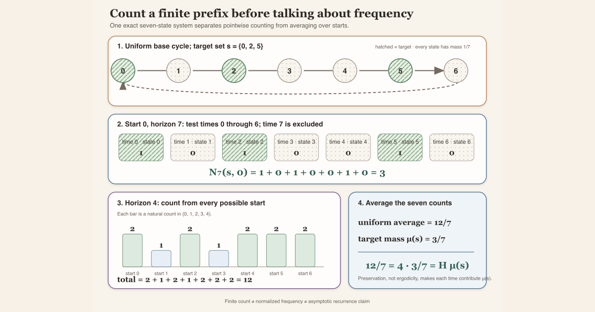
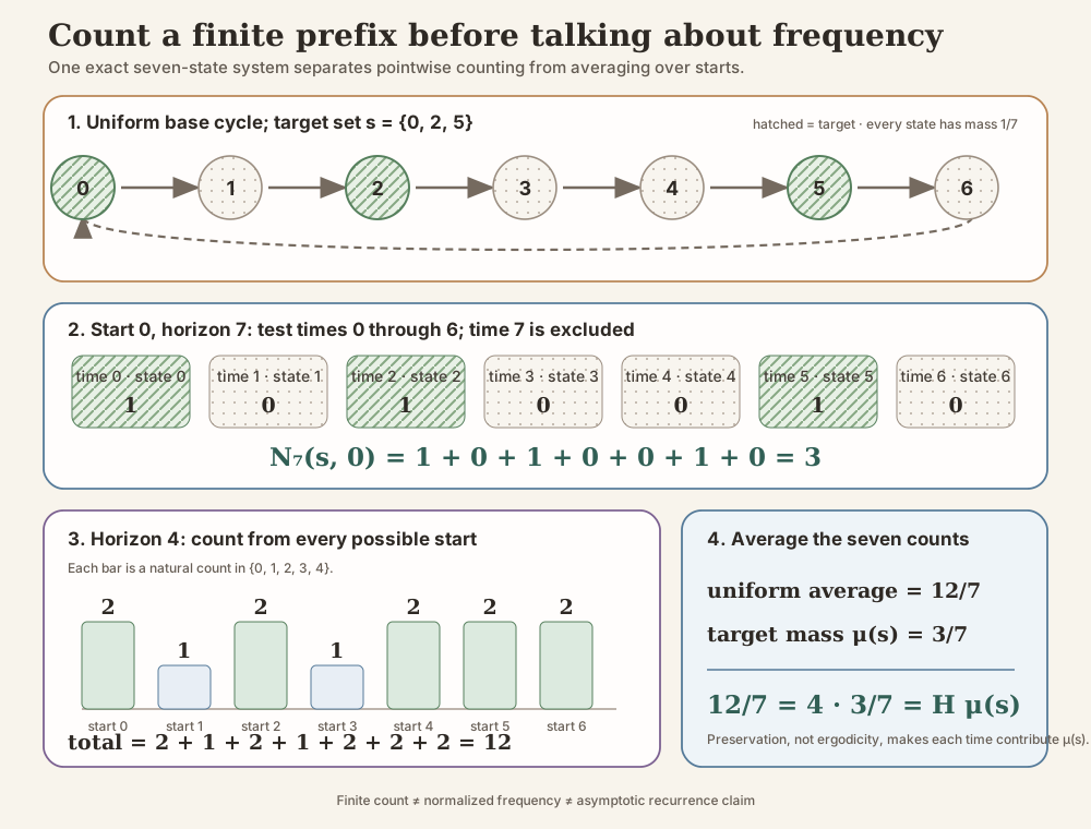
Start with seven states arranged in a cycle:
\[ \Omega=\{0,1,2,3,4,5,6\}, \qquad T(i)=i+1\pmod 7. \]Mark the three-state target set
\[ s=\{0,2,5\}. \]Starting from state \(0\), the first seven orbit positions are
\[ 0,1,2,3,4,5,6. \]Membership in \(s\) produces the indicator list
\[ 1,0,1,0,0,1,0. \]Adding those seven zeros and ones gives
\[ \boxed{N_7(s,0)=1+0+1+0+0+1+0=3}. \]This is a finite orbit visit count. It answers “how many marked positions occur in this particular finite prefix?” It is not yet a percentage, a long-time frequency, or a recurrence theorem.
Define the finite count
Let \(T:\Omega\to\Omega\) be any map, \(s\subseteq\Omega\) any set, \(H\in\mathbb N\) a horizon, and \(\omega\in\Omega\) a starting point. Define
\[ N_H(s,\omega) =\#\{j\in\mathbb N\mid j\lt H\text{ and }T^j\omega\in s\}. \]Read each symbol literally:
- \(T^j\omega\) is the state reached after \(j\) applications of \(T\);
- \(j\lt H\) selects exactly the indices \(0,1,\ldots,H-1\);
- membership \(T^j\omega\in s\) is one yes-or-no test; and
- \(\#\) counts how many indices pass that test.
The value lies in \(\mathbb N\). Two elementary bounds are
\[ 0\le N_H(s,\omega)\le H. \]The upper bound holds because at most all \(H\) tested indices can be visits.
Horizon means number of tested positions
The half-open convention prevents an off-by-one error:
| Horizon | Tested indices | Meaning in the seven-cycle example from start \(0\) | Count |
|---|---|---|---|
| \(0\) | none | empty prefix | \(0\) |
| \(1\) | \(0\) | test the starting state \(0\) | \(1\) |
| \(4\) | \(0,1,2,3\) | visit \(0\), miss \(1\), visit \(2\), miss \(3\) | \(2\) |
| \(7\) | \(0,1,\ldots,6\) | one complete cycle | \(3\) |
Time \(H\) is outside the window. Horizon \(4\) therefore does not test \(T^4(0)=4\).
Repeated visits at different times count separately. If an orbit returns to the same marked state twice within the window, those are two visits because two distinct time indices passed the membership test.
Write the count as an indicator sum
The real-valued indicator of \(s\) is
\[ \mathbf 1_s(x)= \begin{cases} 1,&x\in s,\\ 0,&x\notin s. \end{cases} \]After casting the natural count to \(\mathbb R\), finite counting becomes a Birkhoff sum :
\[ \bigl(N_H(s,\omega):\mathbb R\bigr) =\sum_{j=0}^{H-1}\mathbf 1_s(T^j\omega). \]This equality is finite combinatorics. It needs no measurable space, measure, probability, preservation, or ergodicity. The cast changes the codomain so that real-valued integration can be used later; it does not change the count.
Average over all starts in the seven-cycle
Give every subset of \(\Omega\) the status of an event and put uniform mass \(1/7\) on each state. This is a probability measure . Rotation by one state merely permutes equal masses, so \(T\) is a measure-preserving transformation .
At horizon \(4\), enumerate the four tested states from every possible start:
| Start \(\omega\) | Orbit prefix \(\omega,T\omega,T^2\omega,T^3\omega\) | Indicator list | \(N_4(s,\omega)\) |
|---|---|---|---|
| \(0\) | \(0,1,2,3\) | \(1,0,1,0\) | \(2\) |
| \(1\) | \(1,2,3,4\) | \(0,1,0,0\) | \(1\) |
| \(2\) | \(2,3,4,5\) | \(1,0,0,1\) | \(2\) |
| \(3\) | \(3,4,5,6\) | \(0,0,1,0\) | \(1\) |
| \(4\) | \(4,5,6,0\) | \(0,1,0,1\) | \(2\) |
| \(5\) | \(5,6,0,1\) | \(1,0,1,0\) | \(2\) |
| \(6\) | \(6,0,1,2\) | \(0,1,0,1\) | \(2\) |
The seven counts sum to \(12\), so their uniform average is
\[ \mathbb E[N_4(s,\cdot)] =\frac17(2+1+2+1+2+2+2) =\frac{12}{7}. \]The target set has probability
\[ \mu(s)=\frac37. \]Therefore
\[ \boxed{ \mathbb E[N_4(s,\cdot)] =\frac{12}{7} =4\cdot\frac37 =4\mu(s)}. \]This is not a coincidence special to horizon four. Every tested time has the same probability \(3/7\) of lying in \(s\), because the base preserves the measure. Linearity of the integral then adds \(H\) equal contributions.
The general integral identity
Now let \(\Omega\) carry a measurable structure and a finite measure \(\mu\). Assume that \(T\) preserves \(\mu\) and that \(s\) is null measurable. Then
\[ \boxed{ \int_\Omega \bigl(N_H(s,\omega):\mathbb R\bigr)\,d\mu(\omega) =H\,\mu(s)}. \]The hypotheses have separate jobs:
- Null measurability of \(s\) supplies the measurable representative required for integrating its indicator. It means that \(s\) differs from a measurable set only on a null set .
- Finite total measure makes the bounded indicator integrable.
- Measure preservation makes every shifted indicator \(\mathbf 1_s\circ T^j\) have the same integral \(\mu(s)\).
- Finite horizon reduces the remaining integral to ordinary finite-sum linearity.
Ordinary measurability of \(s\) is sufficient but stronger than required. Ergodicity is not used. On a probability space, the integral is an expectation . For a general finite measure it is an unnormalized integral.
At \(H=0\), both sides are zero. At \(H=1\), the identity reduces to the integral of the target-set indicator.
In Lean: construct the count
finiteOrbitVisitCount T s H ωFinset.range His the finite set of natural numbers belowH.T^[j]is Lean’s notation for thej-fold iterate ofT;T^[j] ωis \(T^j\omega\)..filterkeeps exactly the indices satisfying membership ins..cardreturns the number of retained indices as a natural number.- The definition is
noncomputablebecause membership in an arbitrary mathematical set need not come with a decision procedure.
The exact project definition is:
noncomputable def finiteOrbitVisitCount {Ω : Type uΩ} (T : Ω → Ω)
    (s : Set Ω) (H : ℕ) (ω : Ω) : ℕ := by
  classical
  exact ((Finset.range H).filter fun j ↦ T^[j] ω ∈ s).card
The word classical locally supplies set-membership decisions for
the proof assistant. The mathematical definition remains the finite
cardinality written on paper.
In Lean: turn counting into a Birkhoff sum
natCast_finiteOrbitVisitCount_eq_birkhoffSum_indicator T s H ωnatCastdescribes the coercion from \(\mathbb N\) to \(\mathbb R\).s.indicator fun _ ↦ (1 : ℝ)is the real indicator ofs.birkhoffSum T f H ωmeans∑ j ∈ Finset.range H, f (T^[j] ω).- The theorem has no measurable-space parameter. It is an algebraic identity about a finite sum.
In Lean: integrate the count
integral_finiteOrbitVisitCount hT hs HhT : MeasurePreserving T μ μcertifies measurability and preservation of the same measure.hs : NullMeasurableSet s μis the target-set regularity certificate.[IsFiniteMeasure μ]is a typeclass assumption available to the theorem.μ.real sis Mathlib’s real-valued view of the measure ofs. The theorem’s right side isH * μ.real s.- The result is an equality of real numbers, not an almost-everywhere statement and not a limiting theorem.
The complete exact proof is short because the indicator-sum infrastructure is already available:
theorem integral_finiteOrbitVisitCount
    {Ω : Type uΩ} [MeasurableSpace Ω] {T : Ω → Ω} {μ : Measure Ω}
    [IsFiniteMeasure μ] (hT : MeasurePreserving T μ μ)
    {s : Set Ω} (hs : NullMeasurableSet s μ) (H : ℕ) :
    (∫ ω, (finiteOrbitVisitCount T s H ω : ℝ) ∂μ) =
      H * μ.real s := by
  simp_rw [natCast_finiteOrbitVisitCount_eq_birkhoffSum_indicator]
  rw [integral_birkhoffSum_eq_nat_mul hT
    ((integrable_const (1 : ℝ)).indicator₀ hs) H]
  rw [integral_indicator₀ hs, setIntegral_const]
  simp
The proof first rewrites the count as a Birkhoff sum, integrates the preserved finite sum, evaluates the indicator integral, and simplifies the scalar arithmetic.
Standalone tutorial
Standalone tutorial. The following complete file models
the uniform seven-cycle with natural-number arithmetic only. It imports
Std, not Mathlib or this project.
Save it as OrbitVisitCountScratch.lean:
import Std

namespace OrbitVisitCountScratch

def orbitState (start time : Nat) : Nat :=
  (start + time) % 7

def isTarget (state : Nat) : Bool :=
  state == 0 || state == 2 || state == 5

def visitCount : Nat → Nat → Nat
  | 0, _ => 0
  | horizon + 1, start =>
      visitCount horizon start +
        (if isTarget (orbitState start horizon) then 1 else 0)

def horizonFourCounts : List Nat :=
  (List.range 7).map (visitCount 4)

#eval visitCount 0 0
#eval visitCount 1 0
#eval visitCount 4 0
#eval visitCount 7 0
#eval horizonFourCounts
#eval horizonFourCounts.sum

example : visitCount 7 0 = 3 := by decide
example : horizonFourCounts = [2, 1, 2, 1, 2, 2, 2] := by decide
example : horizonFourCounts.sum = 12 := by decide

end OrbitVisitCountScratch
Run it on macOS or Linux with the pinned Lean toolchain:
elan run leanprover/lean4:v4.32.0 lean OrbitVisitCountScratch.lean
The outputs should be 0, 1, 2,
3, [2, 1, 2, 1, 2, 2, 2], and 12.
Dividing the last result by seven on paper gives the exact expectation
\(12/7\). The worksheet checks the finite combinatorics; the
measure-theoretic identity remains the project theorem checked below.
Try the exact declarations in the project
Full project check. This uses the repository’s pinned Lean and Mathlib dependencies and may require substantial disk space and memory. Ask Lean for the exact declaration types:
import NonlinearDynamics.Random.RandomCocycles.SubadditiveBadBlockMeasure

open MeasureTheory

#check NonlinearDynamics.Random.RandomCocycles.finiteOrbitVisitCount
#check NonlinearDynamics.Random.RandomCocycles.natCast_finiteOrbitVisitCount_eq_birkhoffSum_indicator
#check NonlinearDynamics.Random.RandomCocycles.integral_finiteOrbitVisitCount
#check birkhoffSum
#check birkhoffSum_zero
#check birkhoffSum_succ
#check integral_birkhoffSum_eq_nat_mul
#check MeasurePreserving
#check NullMeasurableSet
Each #check asks the pinned elaborator for an existing type. The
full-project command below checks the complete project module with the
repository’s pinned dependencies installed.
cd formalization
lake env lean -DwarningAsError=true NonlinearDynamics/Random/RandomCocycles/SubadditiveBadBlockMeasure.lean
Resource note: this exact file uses the repository's
pinned Lean and Mathlib dependencies. Initial project setup can require
substantial disk space and build time. For a lightweight first step on
macOS or Linux, use the page's standalone Lean-core or Std
tutorial.
Boundary cases and near-misses
- Empty horizon: \(N_0(s,\omega)=0\) for every set and start because
Finset.range 0is empty. - Empty target: \(N_H(\varnothing,\omega)=0\).
- Whole target: \(N_H(\Omega,\omega)=H\).
- Repeated state: returning to one state at two different indices counts twice; the definition counts indices, not distinct states.
- Time \(H\): a visit exactly at time \(H\) is excluded from the horizon-\(H\) count.
- Natural versus real: the definition returns \(\mathbb N\); only the integral theorem casts it to \(\mathbb R\).
- Measurable but infinite base measure: the exact integral theorem assumes finite total measure so that the bounded indicator is integrable.
- Preservation without ergodicity: the integral identity still holds. Ergodicity is irrelevant to this finite expectation calculation.
What the count does not establish
A finite orbit visit count is not automatically:
- a visit frequency, because it has not been divided by \(H\);
- an asymptotic density, because no limit as \(H\to\infty\) has been taken;
- a recurrence theorem, because one finite window cannot prove infinitely many returns;
- an ergodic theorem, because neither the definition nor the integral identity identifies a long-time limit;
- a probability, because the pointwise count can be any natural number up to \(H\); or
- an independence statement, because successive membership tests come from one orbit and can be strongly dependent.
The seven-cycle happens to be ergodic under its uniform measure, but the finite identity was proved using preservation alone. The example does not justify adding ergodicity to the general statement.
Check your understanding
- With the same seven-cycle and target set, compute \(N_3(s,5)\).
- Why does horizon \(1\) test the starting state rather than \(T\omega\)?
- What are the visit counts when \(s=\varnothing\) and when \(s=\Omega\)?
- Explain why two returns to the same target state count twice.
- Which hypothesis makes \(\int \mathbf 1_s(T^j\omega)\,d\mu=\mu(s)\) independent of \(j\)?
- Why is the integral called an expectation only when the measure has total mass one?
- What additional normalization and limiting theorem would be needed before discussing long-run visit frequency?
Where to continue
The Birkhoff sum entry generalizes the zero-or-one indicator to any real observable. The finite maximal ergodic inequality uses finite orbit sums to control threshold events. The ergodicity entry explains the separate invariant-set rigidity assumption that becomes important for asymptotic identification.
Finite Centered Bad-Block Measure Control in Lean uses visit counts as a combinatorial budget inside a larger subadditive proof. Finite Bad-Block Measure Bounds Before Kingman Lower Liminf develops that argument as a textbook chapter.
Sources
Resource label: pinned project. The repository’s checked RMT-30 module is authoritative for the definition, finite indicator identity, and integral theorem quoted above.
Resource label: pinned Mathlib. The pinned revision supplies the Birkhoff-sum interface, null-measurable indicator integration, and null-measurable function and set APIs used by that proof.
The exact upstream Lean revision audited for this page is Mathlib commit
81a5d257,
the revision pinned by formalization/lake-manifest.json.