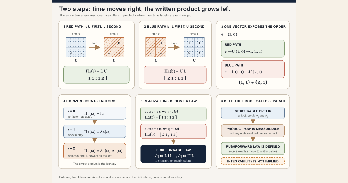
Begin with two concrete \(2\) by \(2\) matrices:
\[ U= \begin{bmatrix} 1&1\\ 0&1 \end{bmatrix}, \qquad L= \begin{bmatrix} 1&0\\ 1&1 \end{bmatrix}. \]The matrix \(U\) is an upper shear and \(L\) is a lower shear. Suppose one sample path, called \(r\), selects
\[ A_0(r)=U, \qquad A_1(r)=L. \]Time \(0\) happens first. Time \(1\) happens second. For column vectors, the first matrix action must therefore be closest to the vector:
\[ x_2=A_1(r)\bigl(A_0(r)x_0\bigr) =\bigl(A_1(r)A_0(r)\bigr)x_0. \]The two-step forward product is consequently
\[ \Pi_2(r)=A_1(r)A_0(r)=LU. \]The newest factor is written on the left.
Calculate both orders
Matrix multiplication is generally noncommutative. Compute the order selected by the time convention:
\[ \begin{aligned} LU &= \begin{bmatrix} 1&0\\ 1&1 \end{bmatrix} \begin{bmatrix} 1&1\\ 0&1 \end{bmatrix}\\ &= \begin{bmatrix} 1\cdot1+0\cdot0 & 1\cdot1+0\cdot1\\ 1\cdot1+1\cdot0 & 1\cdot1+1\cdot1 \end{bmatrix}\\ &= \begin{bmatrix} 1&1\\ 1&2 \end{bmatrix}. \end{aligned} \]Now reverse the order:
\[ \begin{aligned} UL &= \begin{bmatrix} 1&1\\ 0&1 \end{bmatrix} \begin{bmatrix} 1&0\\ 1&1 \end{bmatrix}\\ &= \begin{bmatrix} 1\cdot1+1\cdot1 & 1\cdot0+1\cdot1\\ 0\cdot1+1\cdot1 & 0\cdot0+1\cdot1 \end{bmatrix}\\ &= \begin{bmatrix} 2&1\\ 1&1 \end{bmatrix}. \end{aligned} \]Therefore
\[ LU\ne UL. \]Reversing the written factors changes the matrix. It also changes the chronology. Let
\[ e= \begin{bmatrix} 1\\ 0 \end{bmatrix}. \]Along path \(r\), the intended updates are
\[ e \xrightarrow{\,U\,} \begin{bmatrix}1\\0\end{bmatrix} \xrightarrow{\,L\,} \begin{bmatrix}1\\1\end{bmatrix}. \]Indeed, the first column of \(LU\) is \((1,1)^{\mathsf T}\). Reversing the actions gives
\[ e \xrightarrow{\,L\,} \begin{bmatrix}1\\1\end{bmatrix} \xrightarrow{\,U\,} \begin{bmatrix}2\\1\end{bmatrix}, \]the first column of \(UL\). The order difference is observable on a single vector.
Horizon zero is the identity
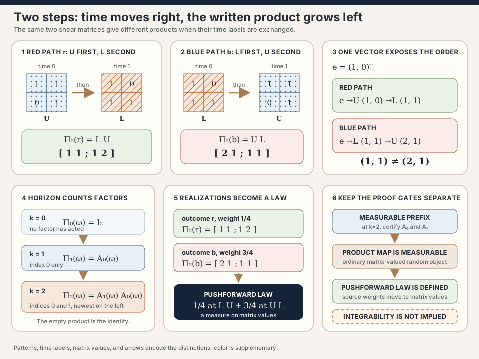
A horizon counts how many factors have acted. It does not name the final index. The first horizons are
\[ \begin{aligned} \Pi_0(\omega)&=I,\\ \Pi_1(\omega)&=A_0(\omega),\\ \Pi_2(\omega)&=A_1(\omega)A_0(\omega),\\ \Pi_3(\omega)&=A_2(\omega)A_1(\omega)A_0(\omega). \end{aligned} \]For our \(2\) by \(2\) paths,
\[ \Pi_0(\omega)= I_2= \begin{bmatrix} 1&0\\ 0&1 \end{bmatrix} \qquad\text{for every }\omega. \]There is no time-zero factor hiding in this expression. Horizon zero uses an empty list of factors, and the product of an empty list is the multiplicative identity. Consequently,
\[ \Pi_0(\omega)x=x. \]This convention makes the successor recursion uniform:
\[ \boxed{ \Pi_{k+1}(\omega)=A_k(\omega)\Pi_k(\omega) }. \]It also makes a split after \(m\) factors work when either block is empty.
Turn the two orders into a random product
Now use the outcome space
\[ \Omega=\{r,b\}. \]The same two matrices appear on both outcomes, but their time order differs:
| Outcome | \(A_0(\omega)\) | \(A_1(\omega)\) | \(\Pi_2(\omega)=A_1(\omega)A_0(\omega)\) |
|---|---|---|---|
| \(r\) | \(U\) | \(L\) | \(LU=\begin{bmatrix}1&1\\1&2\end{bmatrix}\) |
| \(b\) | \(L\) | \(U\) | \(UL=\begin{bmatrix}2&1\\1&1\end{bmatrix}\) |
The entire function
\[ \Pi_2:\Omega\longrightarrow M_2(\mathbb R) \]is the two-step sample-product map. Applying it to one outcome gives one realization. For example,
\[ \Pi_2(r)= \begin{bmatrix} 1&1\\ 1&2 \end{bmatrix} \]is one ordinary matrix. It is not a probability measure. For the project’s complex-matrix law, these real entries are regarded as complex numbers with zero imaginary part.
Give the outcomes probabilities
\[ \mu\{r\}=\frac14, \qquad \mu\{b\}=\frac34. \]The probability law of the product map is the measure on matrix space
\[ \begin{aligned} \mathcal L_\mu(\Pi_2) &=\frac14\, \delta_{\left[\begin{smallmatrix}1&1\\1&2\end{smallmatrix}\right]}\\ &\quad+\frac34\, \delta_{\left[\begin{smallmatrix}2&1\\1&1\end{smallmatrix}\right]}. \end{aligned} \]The symbol \(\delta_M\) denotes a point mass at matrix \(M\). For instance, let \(E\) be the set of matrices whose upper-left entry is \(1\). Only the red product lies in \(E\), so
\[ \mathcal L_\mu(\Pi_2)(E) =\mu\{\omega:\Pi_2(\omega)\in E\} =\mu\{r\} =\frac14. \]The realized matrix answers “what product occurred on this path?” The law answers “how is probability distributed over all possible product values?” Changing the source weights changes the law without changing either matrix formula.
The factors in this toy model are not independent: once the outcome is known, the entire two-step order is known. Independence is not required to define a finite sample product or its pushforward law.
The general pointwise construction
Let \(\Omega\) be an outcome type and let
\[ A_j:\Omega\longrightarrow M_\iota(\mathbb K) \]be a square matrix-valued map at every natural time \(j\). The project first defines the deterministic ordered product
\[ P_B(0)=I, \qquad P_B(k+1)=B_kP_B(k). \]It then substitutes \(B_j=A_j(\omega)\):
\[ \Pi_k(\omega)=P_{j\mapsto A_j(\omega)}(k). \]This algebraic construction needs a finite matrix index type and semiring scalars. A semiring supplies the finite sums, products, zero, and identity used in matrix multiplication. It needs no measurable space, measure, probability, independence, norm, or integral.
Splitting after \(m\) factors gives
\[ \Pi_{m+k}(\omega) =\Pi^{(m)}_k(\omega)\Pi_m(\omega), \]where \(\Pi^{(m)}_k\) uses the shifted factors \(j\mapsto A_{m+j}\). The later block is on the left because it acts after the earlier block.
Exact prefix measurability
To form the ordinary pushforward law in the intended regime, the map \(\Pi_k\) must be measurable . The checked hypothesis is exactly
\[ \forall j\lt k,\quad A_j\text{ is measurable}. \]At horizon \(2\), only \(A_0\) and \(A_1\) appear. The measurability of \(A_2,A_3,\ldots\) is irrelevant. At horizon \(0\), the condition is vacuous because there is no natural number \(j\lt0\).
The proof mirrors the recursion:
- \(\Pi_0\) is the constant identity map, hence measurable.
- If \(A_k\) and \(\Pi_k\) are measurable, then \(\omega\mapsto A_k(\omega)\Pi_k(\omega)\) is measurable.
- Induction reaches every finite horizon.
Why is matrix multiplication measurable? Each output entry is a finite sum
\[ (XY)_{rc}=\sum_s X_{rs}Y_{sc} \]of products of measurable complex coordinate functions. The shared index type is finite, so the sum has finitely many terms.
On the finite two-outcome space above, give every subset of \(\Omega\) the status of an event. Every map out of that discrete measurable space is measurable, which supplies the prefix certificate.
Measurability is not integrability
Measurability asks whether target events have allowed source preimages. Integrability asks whether a measurable quantity has finite total norm under a chosen measure. The first property does not provide the second.
There is an even sharper product warning. On the probability space \((0,1]\) with Lebesgue measure, set
\[ D(t)= \begin{bmatrix} t^{-1/2}&0\\ 0&1 \end{bmatrix} \qquad(0\lt t\le1). \]Use \(A_0(t)=A_1(t)=D(t)\). For the maximum absolute row-sum norm,
\[ \lVert D(t)\rVert=t^{-1/2}, \]and
\[ \int_0^1 t^{-1/2}\,dt=2. \]Thus each factor has integrable norm. But
\[ \Pi_2(t)=D(t)^2= \begin{bmatrix} t^{-1}&0\\ 0&1 \end{bmatrix}, \qquad \lVert\Pi_2(t)\rVert=t^{-1}, \]and
\[ \int_0^1 t^{-1}\,dt=\infty. \]Even integrability of each one-step norm does not automatically imply integrability of their product. Boundedness, independence plus suitable moments, or a direct domination argument could supply additional control, but none is present in the finite-product measurability module. This calculus example explains the boundary; it is not a theorem formalized in that module.
Measurability itself does not mention the source measure. Integrability is always relative to a measure. That type-level separation is deliberate.
From a measurable sample map to its law
Let \(\mu\) be a measure on \(\Omega\). Once \(\Pi_k\) is measurable, the project defines
\[ \mathcal L_\mu(\Pi_k) =(\Pi_k)_*\mu, \]the pushforward of \(\mu\) through the sample-product map. For every measurable matrix set \(S\),
\[ \mathcal L_\mu(\Pi_k)(S) =\mu\{\omega:\Pi_k(\omega)\in S\}. \]Mathlib’s Measure.map is total: outside its
almost-everywhere-measurable branch it falls back to the zero measure. The
project’s RandomMatrix.law wrapper therefore receives an explicit
ordinary measurability proof. That proof records why this use of
Measure.map has the intended pushforward meaning.
The raw forwardProductLaw accepts any source
Measure Ω. If \(\mu\) is a
probability measure
, the project proves
that the result also has total mass one. It can then be bundled as a
ProbabilityMeasure. The wrapper changes what the type records;
it does not change any event probabilities.
At horizon zero, under a probability source,
\[ \mathcal L_\mu(\Pi_0)=\delta_I. \]At horizon one,
\[ \mathcal L_\mu(\Pi_1)=\mathcal L_\mu(A_0). \]The zero-horizon Dirac formula uses probability normalization. Pushing an arbitrary measure through a constant identity map preserves its total mass, which need not be one.
In Lean
The successor equation translates chronological action into Lean syntax.
sampleForwardProduct A (k + 1) = fun ω => A k ω * sampleForwardProduct A k ωsampleForwardProductis the outcome-to-product map.Ais a time-indexed family. ThusA kis the map at timek, andA k ωis its realized matrix at outcomeω.k + 1is the successor horizon. Its newest factor has indexk.fun ω =>constructs a function of the outcome. It corresponds to the paper notation \(\omega\mapsto\cdots\).*is matrix multiplication. Its operand order is literal.- The equality is an equality of functions, not merely an equality at one chosen outcome.
These are exact declarations from the checked project module:
def sampleForwardProduct (A : ℕ → RandomMatrix Ω ι ι 𝕜) (k : ℕ) :
    RandomMatrix Ω ι ι 𝕜 :=
  fun ω => forwardProduct (fun j => A j ω) k

@[simp] theorem sampleForwardProduct_zero (A : ℕ → RandomMatrix Ω ι ι 𝕜) :
    sampleForwardProduct A 0 = fun _ => 1 := rfl

@[simp] theorem sampleForwardProduct_succ
    (A : ℕ → RandomMatrix Ω ι ι 𝕜) (k : ℕ) :
    sampleForwardProduct A (k + 1) =
      fun ω => A k ω * sampleForwardProduct A k ω := rfl
The symbol 1 is the matrix identity because Lean infers its type
from the surrounding matrix-valued function. The proof rfl
means that the zero and successor equations follow by unfolding the recursive
definitions.
The exact-prefix theorem keeps every used assumption visible:
measurable_sampleForwardProduct A k hAhAis proof evidence with type∀ j < k, Measurable (A j).∀means “for every,” andj < kselects exactly the finite prefix of indices \(0,\ldots,k-1\).Measurable (A j)concerns one matrix-valued factor map.- The conclusion
Measurable (sampleForwardProduct A k)concerns the whole finite product map. - The strict comparison is typed literally as
<in Lean code. Paper mathematics on this site uses \(\lt\) inside TeX.
Here is the exact theorem and proof:
theorem measurable_sampleForwardProduct (A : ℕ → RandomMatrix Ω ι ι ℂ)
    (k : ℕ) (hA : ∀ j < k, Measurable (A j)) :
    Measurable (sampleForwardProduct A k) := by
  induction k with
  | zero =>
      rw [sampleForwardProduct_zero]
      exact RandomMatrix.measurable_const 1
  | succ k ih =>
      rw [sampleForwardProduct_succ]
      exact RandomMatrix.measurable_mul
        (hA k (Nat.lt_succ_self k))
        (ih fun j hj => hA j (Nat.lt_succ_of_lt hj))
The zero branch proves measurability of the constant identity.
The succ branch obtains the newest factor from hA,
uses the induction hypothesis for the earlier prefix, and applies measurable
matrix multiplication.
Finally, the law constructor receives that certificate:
forwardProductLaw μ A k hAμ : Measure Ωis the source measure.A,k, andhAspecify the same certified sample-product map as above.- The result has type
Measure (Matrix ι ι ℂ). It is a measure on matrix values, not another matrix and not a function on outcomes. - If
μhas a probability-measure instance, a separate theorem proves that this raw law has total mass one.
The exact definition is:
noncomputable def forwardProductLaw (μ : Measure Ω)
    (A : ℕ → RandomMatrix Ω ι ι ℂ)
    (k : ℕ) (hA : ∀ j < k, Measurable (A j)) :
    Measure (Matrix ι ι ℂ) :=
  RandomMatrix.law (sampleForwardProduct A k)
    (measurable_sampleForwardProduct A k hA) μ
The word noncomputable says that Lean is defining a classical
mathematical object rather than executable code. It does not weaken the
definition or introduce an unproved proposition.
A tiny standalone worksheet
The following complete Lean program uses only Std. It implements
integer \(2\) by \(2\) multiplication and folds a chronological list
[A₀, A₁, …] by placing each newest factor on the left.
Save it as FiniteProductWorksheet.lean:
import Std

namespace FiniteProductWorksheet

structure Mat2 where
  a00 : Int
  a01 : Int
  a10 : Int
  a11 : Int
deriving Repr, DecidableEq

def matMul (X Y : Mat2) : Mat2 :=
  { a00 := X.a00 * Y.a00 + X.a01 * Y.a10
  , a01 := X.a00 * Y.a01 + X.a01 * Y.a11
  , a10 := X.a10 * Y.a00 + X.a11 * Y.a10
  , a11 := X.a10 * Y.a01 + X.a11 * Y.a11 }

def identity : Mat2 :=
  { a00 := 1, a01 := 0, a10 := 0, a11 := 1 }

def upperShear : Mat2 :=
  { a00 := 1, a01 := 1, a10 := 0, a11 := 1 }

def lowerShear : Mat2 :=
  { a00 := 1, a01 := 0, a10 := 1, a11 := 1 }

def lowerAfterUpper : Mat2 :=
  { a00 := 1, a01 := 1, a10 := 1, a11 := 2 }

def upperAfterLower : Mat2 :=
  { a00 := 2, a01 := 1, a10 := 1, a11 := 1 }

def forwardProduct (factors : List Mat2) : Mat2 :=
  factors.foldl (fun earlier newest => matMul newest earlier) identity

inductive Outcome where
  | red
  | blue
deriving Repr, DecidableEq

def samplePath : Outcome → List Mat2
  | .red => [upperShear, lowerShear]
  | .blue => [lowerShear, upperShear]

def realizedProduct (ω : Outcome) : Mat2 :=
  forwardProduct (samplePath ω)

#eval matMul lowerShear upperShear
#eval matMul upperShear lowerShear
#eval realizedProduct .red
#eval realizedProduct .blue
#eval forwardProduct []

example : matMul lowerShear upperShear = lowerAfterUpper := by decide
example : matMul upperShear lowerShear = upperAfterLower := by decide
example : lowerAfterUpper ≠ upperAfterLower := by decide
example : realizedProduct .red = lowerAfterUpper := by decide
example : realizedProduct .blue = upperAfterLower := by decide
example : forwardProduct [] = identity := by decide

end FiniteProductWorksheet
With Elan installed, a human opens a terminal in the directory containing the file and types:
elan run leanprover/lean4:v4.32.0 lean FiniteProductWorksheet.lean
Lean prints the two distinct products twice, once by direct multiplication and
once through the two sample paths, then prints the identity for the empty
list. The six example declarations ask the Lean kernel to certify
the calculations and noncommutativity.
This worksheet is a small executable model. It does not import Mathlib, define measurable spaces or measures, or construct the weighted law \(\frac14\delta_{LU}+\frac34\delta_{UL}\).
The checked project layer
Full project check. This uses the repository’s pinned Lean and Mathlib dependencies and may require substantial disk space and memory.
The authoritative algebraic source is formalization/NonlinearDynamics/Random/MatrixProducts/FiniteProducts.lean. The sample-map and law source is formalization/NonlinearDynamics/Random/MatrixProducts/MeasurableFiniteProducts.lean.
A learner can place the following exact lines in a temporary scratch file
inside the formalization project:
import NonlinearDynamics.Random.MatrixProducts.MeasurableFiniteProducts

open Matrix MeasureTheory

#check NonlinearDynamics.Random.MatrixProducts.forwardProduct
#check NonlinearDynamics.Random.MatrixProducts.forwardProduct_zero
#check NonlinearDynamics.Random.MatrixProducts.forwardProduct_succ
#check NonlinearDynamics.Random.MatrixProducts.forwardProduct_add
#check NonlinearDynamics.Random.MatrixProducts.sampleForwardProduct
#check NonlinearDynamics.Random.MatrixProducts.sampleForwardProduct_zero
#check NonlinearDynamics.Random.MatrixProducts.sampleForwardProduct_succ
#check NonlinearDynamics.Random.MatrixProducts.measurable_sampleForwardProduct
#check NonlinearDynamics.Random.MatrixProducts.forwardProductLaw
#check NonlinearDynamics.Random.MatrixProducts.forwardProductLaw_zero
#check NonlinearDynamics.Random.MatrixProducts.forwardProductLaw_one
#check NonlinearDynamics.Random.MatrixProducts.forwardProductProbabilityLaw
import loads the checked project module and its pinned Mathlib
dependencies. Each #check asks Lean to elaborate one declaration
and print its type. It does not create a theorem or evaluate the toy matrices.
To check the authoritative module itself from the repository root, type:
cd formalization
lake env lean NonlinearDynamics/Random/MatrixProducts/MeasurableFiniteProducts.lean
cd formalization
lake env lean -DwarningAsError=true NonlinearDynamics/Random/MatrixProducts/MeasurableFiniteProducts.lean
Resource note: this exact file uses the repository's
pinned Lean and Mathlib dependencies. Initial project setup can require
substantial disk space and build time. For a lightweight first step on
macOS or Linux, use the page's standalone Lean-core or Std
tutorial.
Distinctions and boundary cases
| Do not confuse | With | Why the difference matters |
|---|---|---|
| Time order \(A_0\) then \(A_1\) | Written order \(A_1A_0\) | The earliest factor acts first on a column vector but is written furthest right |
| Horizon \(k\) | Largest factor index \(k\) | Horizon \(k\) uses indices \(0,\ldots,k-1\) |
| One realization \(\Pi_k(\omega)\) | The sample-product map \(\Pi_k\) | The first is one matrix; the second is a function from all outcomes |
| Sample-product map \(\Pi_k\) | Its law \((\Pi_k)_*\mu\) | The first returns matrices; the second assigns mass to measurable matrix sets |
| Measurability | Integrability | Allowed preimages do not imply finite expected norm |
| Integrable one-step norms | An integrable product norm | The \(D(t)\) example has two integrable factors but a nonintegrable product |
| A finite product | An infinite product or asymptotic rate | No limit follows from a fixed finite horizon |
| A law | Independence or identical distribution | Pushforward construction needs neither property |
| Raw measure | Bundled probability measure | The latter carries total-mass-one evidence in its type |
The matrix index type may be empty. There is still one empty square matrix, so
the identity, multiplication, sample product, measurability theorem, and law
remain meaningful without a Nonempty ι assumption. Positive
dimension enters the companion operator-norm layer because its normalized
identity theorem needs it, not because the algebraic product fails.
If the source measure has zero mass, every pushforward law has zero mass. If the source is a Dirac measure at one outcome, the product law is a Dirac measure at that outcome’s realized product. Neither boundary changes the pointwise product formula.
Where to continue
The forward matrix product page develops the deterministic order and split identities. The random matrix page separates a matrix-valued function from one realization. The measurable function , pushforward measure , and probability law pages develop the three measure-theoretic layers used here. Read integrability for the finite-size condition that this module deliberately does not supply.
Measurable Finite Random-Matrix Products and Proof-Carrying Pushforward Laws audits every declaration in the checked source. Generator-Presented One-Sided Discrete Matrix Cocycles adds one measurable generator along a base orbit and proves the corresponding finite cocycle identity. The one-sided discrete matrix cocycle glossary entry gives the intermediate concept.
References
Mathlib contributors.
Pushforward of a measure,
Mathlib 4 documentation. This official implementation reference defines
Measure.map and its measurable-map evaluation theorem.
Mathlib contributors.
Bundled probability measures,
Mathlib 4 documentation. This source defines ProbabilityMeasure
and its coercion to raw measures.
Olav Kallenberg. Foundations of Modern Probability, third edition, Springer, 2021. This is a standard reference for measurable random elements, pushforward distributions, and integration.
Ludwig Arnold. Random Dynamical Systems, Springer Monographs in Mathematics, 1998. This develops the later cocycle and ergodic setting in which long random matrix products are studied. Those structures motivate the finite interface but are not claims of this page.
The local project uses Mathlib 4.32.0 pinned at commit 81a5d257.