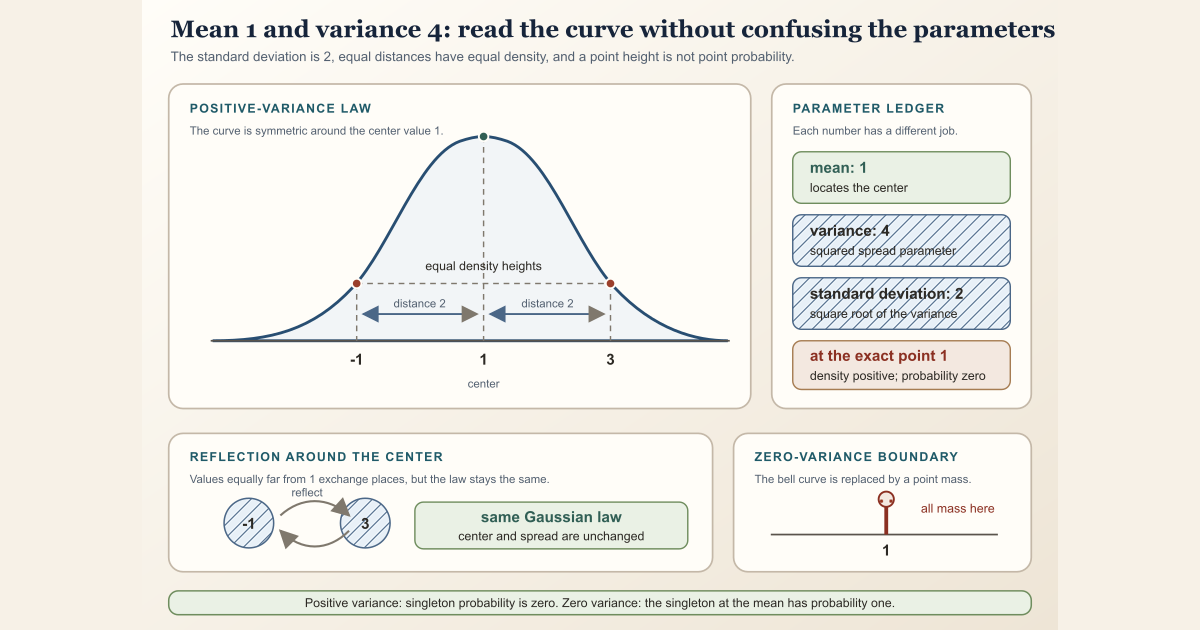
A Gaussian distribution, also called a normal distribution, is a probability law on the real line. Its mean chooses the center. Its variance chooses the squared scale of its spread.
Those two sentences become concrete in the example
\[ X\sim\gamma_{1,4}, \]meaning that \(X\) has Gaussian mean \(1\) and variance \(4\).
Start with mean 1 and variance 4
The center is the mean:
\[ m=1. \]The standard deviation is the nonnegative square root of the variance:
\[ \sigma=\sqrt v=\sqrt4=2. \]Thus the two points one standard deviation from the center are
\[ 1-2=-1 \qquad\text{and}\qquad 1+2=3. \]Because the variance is positive, this law has density
\[ f(x) =\frac{1}{2\sqrt{2\pi}} \exp\!\left(-\frac{(x-1)^2}{8}\right). \]The density depends on \(x\) only through the squared distance \((x-1)^2\). The two one-standard-deviation points are equally far from the center:
\[ (-1-1)^2=4=(3-1)^2. \]Therefore
\[ f(-1)=f(3) =\frac{e^{-1/2}}{2\sqrt{2\pi}}. \]This is an exact symmetry calculation, not a visual guess from a bell-shaped curve.
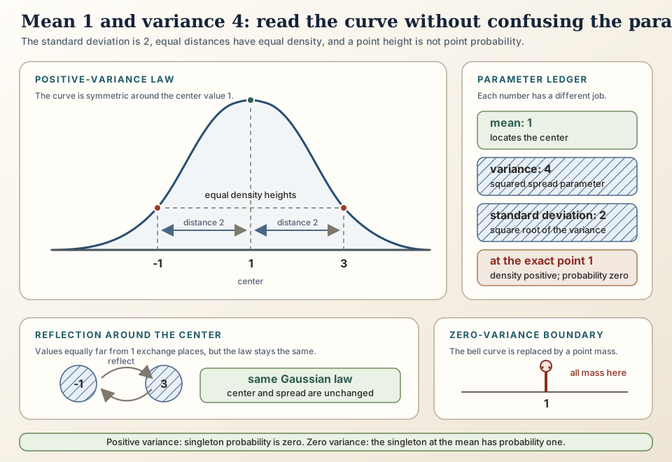
Build the example by an affine transformation
Let \(Z\sim\gamma_{0,1}\) be standard Gaussian and define
\[ X=1+2Z. \]The mean transforms linearly:
\[ \mathbb E[X] =1+2\mathbb E[Z] =1. \]Variance ignores the translation and squares the scale factor:
\[ \operatorname{Var}(X) =2^2\operatorname{Var}(Z) =4. \]Hence
\[ 1+2Z\sim\gamma_{1,4}. \]Reflection around the center gives another useful check. Since \(-Z\sim\gamma_{0,1}\),
\[ 2-X=2-(1+2Z)=1-2Z\sim\gamma_{1,4}. \]So \(X\) and \(2-X\) have the same law. This is distributional symmetry about \(1\); it does not say that \(X(\omega)=2-X(\omega)\) for every outcome.
Variance is not standard deviation
For \(\gamma_{1,4}\),
| Quantity | Value | Role |
|---|---|---|
| Mean \(m\) | \(1\) | center |
| Variance \(v\) | \(4\) | expected squared spread |
| Standard deviation \(\sigma=\sqrt v\) | \(2\) | spread in the same units as \(X\) |
The distinction matters under rescaling. If \(Y=cX\), then
\[ \operatorname{Var}(Y)=c^2\operatorname{Var}(X), \qquad \operatorname{sd}(Y)=|c|\operatorname{sd}(X). \]A factor of \(3\) multiplies standard deviation by \(3\) but variance by
\(9\). The second argument of Mathlib’s gaussianReal m v is
variance \(v\), not standard deviation.
Notation in books and software is not universal. An author may write \(N(m,\sigma^2)\), \(N(m,v)\), or even use the second slot for \(\sigma\). Always inspect the stated convention rather than guessing from the letter.
Density height is not probability
The opening density has a positive height at its center:
\[ f(1)=\frac{1}{2\sqrt{2\pi}}\gt0. \]But \(f(1)\) is probability per unit length, not \(\mathbb P(X=1)\). For a positive-variance Gaussian,
\[ \mathbb P(X=1)=0. \]The singleton \(\{1\}\) is a null set for this law even though \(1\) is the most likely location in the density-height sense.
An interval has probability obtained by integrating density:
\[ \mathbb P(a\le X\le b) =\int_a^b f(x)\,dx. \]Changing an interval’s width changes its probability. A point has width zero, so reading a curve height as point probability is a category mistake.
The general real Gaussian law
This page writes the Gaussian law with mean \(m\in\mathbb R\) and nonnegative variance \(v\) as
\[ \gamma_{m,v}. \]For \(v\gt0\), its density is
\[ f_{m,v}(x) =\frac{1}{\sqrt{2\pi v}} \exp\!\left(-\frac{(x-m)^2}{2v}\right), \qquad x\in\mathbb R. \]The density is nonnegative and integrates to one. Its symmetry is
\[ f_{m,v}(m-t)=f_{m,v}(m+t) \]for every real displacement \(t\).
Every such law can be built from a standard Gaussian \(Z\) by
\[ X=m+\sqrt v\,Z. \]Scaling sets the variance, while translation sets the mean:
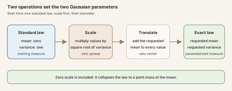
Zero variance is a Dirac law, not a broken density
The formula containing \(1/\sqrt v\) cannot be evaluated by substituting \(v=0\). The exact zero-variance definition is instead
\[ \gamma_{m,0}=\delta_m, \]where \(\delta_m\) is the Dirac probability measure concentrated at \(m\). For every measurable set \(A\subseteq\mathbb R\),
\[ \delta_m(A)= \begin{cases} 1,&m\in A,\\ 0,&m\notin A. \end{cases} \]Thus a random variable with law \(\gamma_{m,0}\) equals \(m\) almost everywhere under its base measure. In particular,
\[ \gamma_{1,0}(\{1\})=1, \]whereas \(\gamma_{1,4}(\{1\})=0\). This boundary is part of the formalized family, not an informal limiting afterthought.
A sample, a law, and Gaussianity are different layers
A random variable \(X:\Omega\to\mathbb R\) is a measurable map from outcomes to values. Its probability distribution, or law under a probability measure \(P\) is the pushforward \(P\circ X^{-1}\).
The exact statement
\[ \mathcal L_P(X)=\gamma_{m,v} \]identifies that complete law. It is much stronger than saying that a finite histogram looks bell-shaped. A finite dataset may support a model check or parameter estimate, but it is not itself a proof of an exact Gaussian law.
The qualitative phrase “\(X\) is Gaussian” also omits information. It says that some Gaussian law is present; it does not itself retain chosen parameters \(m\) and \(v\). The project states the exact parameterized law first and passes to qualitative Gaussianity only through a separate theorem.
In Lean: state the exact parameterized law
HasRealGaussianLaw X 1 4 PX : Ω → ℝmaps an outcome to a real value.P : Measure Ωis the base measure on outcomes.- The numeral
1fills the real mean parameter. - The numeral
4fills a value of typeℝ≥0, also calledNNReal. The type prevents negative variances. HasRealGaussianLawexpands toHasLaw X (gaussianReal 1 4) P.HasLawrecords almost-everywhere measurability ofXand equality between the pushforward law ofXand the stated Gaussian measure. It does not silently upgradeXto ordinary measurability.
Inside the NonlinearDynamics.Random namespace, the exact project
definition is:
def HasRealGaussianLaw (X : Ω → ℝ) (m : ℝ) (v : ℝ≥0)
    (P : Measure Ω) : Prop :=
  HasLaw X (gaussianReal m v) P
Inside its nested HasRealGaussianLaw namespace, the checked
scaling theorem makes the variance square explicit:
theorem const_mul (hX : HasRealGaussianLaw X m v P) (c : ℝ) :
    HasRealGaussianLaw (fun ω ↦ c * X ω) (c * m)
      (⟨c ^ 2, sq_nonneg c⟩ * v) P :=
  gaussianReal_const_mul hX c
If \(m=0\), \(v=1\), and \(c=2\), the result has mean \(0\) and variance \(2^2\cdot1=4\). A subsequent translation changes the mean to \(1\) without changing that variance.
In Lean: preserve the zero-variance boundary
hX.ae_eq_const_of_variance_zerohX : HasRealGaussianLaw X m 0 Pis the exact zero-variance law hypothesis.X =ᵐ[P] fun _ ↦ mis the theorem’s conclusion. The symbol=ᵐ[P]means equality almost everywhere with respect toP.fun _ ↦ mis Lean’s constant function with valuem.- The proof uses Mathlib’s exact identity
gaussianReal_zero_var, which rewrites the law as a Dirac measure.
The zero-variance theorem in that same nested namespace is:
theorem ae_eq_const_of_variance_zero
    (hX : HasRealGaussianLaw X m 0 P) :
    X =ᵐ[P] fun _ ↦ m := by
  apply ProbabilityTheory.HasLaw.ae_eq_of_dirac
  simpa only [HasRealGaussianLaw, gaussianReal_zero_var] using hX
Try the parameter arithmetic locally with Lean and Std
This tiny worksheet checks only the integer parameter bookkeeping for an
affine map \(x\mapsto ax+b\). It imports Std, not Mathlib, and is
safe on an ordinary Mac or Linux machine.
Save it as GaussianParameterTutorial.lean outside the project’s
formalization/ directory:
import Std

structure GaussianParams where
  mean : Int
  variance : Nat
  deriving DecidableEq, Repr

def affineParams (a b : Int) (p : GaussianParams) : GaussianParams :=
  { mean := a * p.mean + b
    variance := Int.natAbs (a * a) * p.variance }

def standard : GaussianParams :=
  { mean := 0, variance := 1 }

def meanOneVarianceFour : GaussianParams :=
  { mean := 1, variance := 4 }

#eval affineParams 2 1 standard
#eval affineParams (-1) 2 meanOneVarianceFour
#eval affineParams 0 7 standard

example : affineParams 2 1 standard = meanOneVarianceFour := by decide
example : affineParams (-1) 2 meanOneVarianceFour =
    meanOneVarianceFour := by decide
example : affineParams 0 7 standard =
    { mean := 7, variance := 0 } := by decide
Run it with the pinned compiler:
elan run leanprover/lean4:v4.32.0 lean GaussianParameterTutorial.lean
The first result is mean \(1\), variance \(4\). The second checks that reflection \(x\mapsto2-x\) preserves those two parameters. The third checks that zero scaling produces mean \(7\), variance \(0\). This worksheet does not construct probability measures or prove that transformed laws are Gaussian; the project and pinned Mathlib declarations below carry those obligations.
Try the exact project interfaces
The following worksheet imports the checked project module. The first block
names project-owned declarations from
NonlinearDynamics/Random/GaussianPrimitives.lean:
import NonlinearDynamics.Random.GaussianPrimitives

open MeasureTheory ProbabilityTheory
open scoped NNReal ProbabilityTheory
open NonlinearDynamics.Random

#check HasRealGaussianLaw
#check HasRealGaussianLaw.mean_eq
#check HasRealGaussianLaw.variance_eq
#check HasRealGaussianLaw.const_mul
#check HasRealGaussianLaw.ae_eq_const_of_variance_zero
#check HasRealGaussianLaw.zero_variance_iff
The imported pinned Mathlib layer supplies the underlying measure and affine transformation facts:
#check gaussianReal
#check gaussianReal_zero_var
#check gaussianReal_map_const_add
#check gaussianReal_map_const_mul
#check nullSingletonClass_gaussianReal
The project checks separate exact law, mean, variance, scaling, and the degenerate boundary. The upstream checks expose the measure constructor, translation and scaling pushforwards, the Dirac identity, and the positive-variance singleton-null property.
cd formalization
lake env lean -DwarningAsError=true NonlinearDynamics/Random/GaussianPrimitives.lean
Resource note: this exact file uses the repository's
pinned Lean and Mathlib dependencies. Initial project setup can require
substantial disk space and build time. For a lightweight first step on
macOS or Linux, use the page's standalone Lean-core or Std
tutorial.
Boundaries that prevent common mistakes
| Tempting claim | Correct statement |
|---|---|
| “Variance \(4\) means standard deviation \(4\).” | Standard deviation is \(\sqrt4=2\). |
| “The density at \(1\) is the probability that \(X=1\).” | Density is a height; the positive-variance singleton probability is zero. |
| “The density formula works at variance zero.” | The zero-variance law is defined separately as \(\delta_m\). |
| “Equal mean and variance determine any probability law.” | They determine the law only after Gaussianity is known. |
| “A bell-shaped histogram proves an exact Gaussian law.” | A finite sample cannot identify the complete law by appearance alone. |
| “Gaussian marginals determine a joint Gaussian law.” | Dependence and the full joint law remain separate data. |
| “HasLaw gives ordinary measurability.” | It supplies almost-everywhere measurability under the base measure. |
Where to continue
Read
variance
for squared-spread calculations,
expectation
for the mean as an integral, and
independence
before combining Gaussian
coordinates. The
Gaussian Laws, Independence, and Normalization
chapter builds finite product laws from these primitives. Continue to
Complex Gaussian Coordinates and Geometry
to join two exact real coordinates without hiding their variance split. The
probability distribution
and
pushforward measure
entries explain
the measure-theoretic level beneath HasLaw.
References
National Institute of Standards and Technology. Normal Distribution, Engineering Statistics Handbook. This official reference states the positive-variance density and distinguishes location from scale.
Mathlib contributors.
Gaussian distributions over the reals,
Mathlib 4 documentation. This is the official API reference for
gaussianReal, its zero-variance Dirac branch, singleton-null
property, and affine transformations.
Mathlib contributors.
Gaussian random variables,
Mathlib 4 documentation. This documents the qualitative
HasGaussianLaw interface.
Project source. GaussianPrimitives.lean defines the exact parameterized law and proves its mean, variance, integrability, scaling, independent-sum, product-family, and zero-variance interfaces.
The project is pinned to Mathlib commit
81a5d257,
so the imported declaration names can be audited against that exact source.