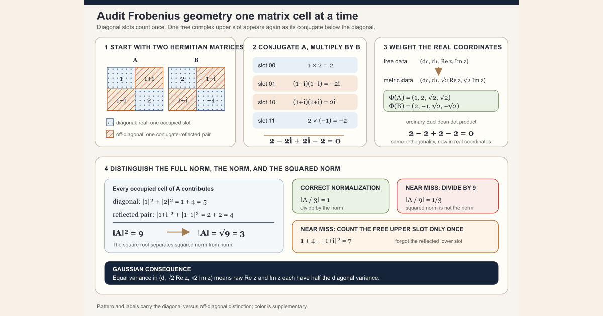
Start with two concrete matrices:
\[ A= \begin{bmatrix} 1 & 1+i\\ 1-i & 2 \end{bmatrix}, \qquad B= \begin{bmatrix} 2 & 1-i\\ 1+i & -1 \end{bmatrix}. \]Both are Hermitian . Their diagonal entries are real, and each lower-left entry is the complex conjugate of the upper-right entry. We will use these two matrices to compute the geometry before introducing its general notation.
Multiply matching entries, then add
For complex matrices, the Frobenius inner product conjugates each entry of the first matrix, multiplies by the matching entry of the second matrix, and adds every result:
\[ \langle A,B\rangle_F =\sum_{r,c}\overline{A_{rc}}\,B_{rc}. \]Here is the complete \(2\) by \(2\) ledger. No entry is hidden.
| Position | \(\overline{A_{rc}}\) | \(B_{rc}\) | Contribution |
|---|---|---|---|
| \((0,0)\) | \(1\) | \(2\) | \(2\) |
| \((0,1)\) | \(1-i\) | \(1-i\) | \((1-i)^2=-2i\) |
| \((1,0)\) | \(1+i\) | \(1+i\) | \((1+i)^2=2i\) |
| \((1,1)\) | \(2\) | \(-1\) | \(-2\) |
Adding the last column gives
\[ \langle A,B\rangle_F =2-2i+2i-2 =0. \]The matrices are therefore orthogonal in Frobenius geometry. Orthogonal does not mean that their entries are disjoint or individually zero. It means that all entrywise contributions cancel in the inner product.
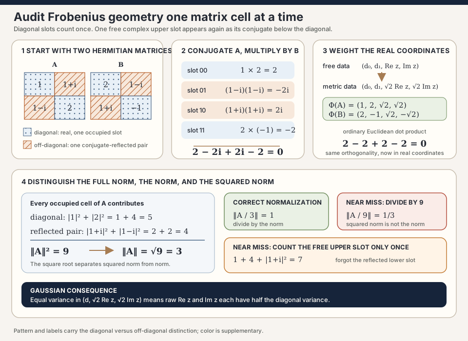
Compute the norm, and avoid two near misses
The Frobenius norm comes from the inner product:
\[ \lVert A\rVert_F^2 =\langle A,A\rangle_F =\sum_{r,c}|A_{rc}|^2. \]For \(A\), the four entry contributions are
\[ |1|^2=1,\qquad |1+i|^2=2,\qquad |1-i|^2=2,\qquad |2|^2=4. \]Thus
\[ \lVert A\rVert_F^2=1+2+2+4=9, \qquad \lVert A\rVert_F=\sqrt9=3. \]The same calculation gives \(\lVert B\rVert_F^2=9\). Consequently
\[ \begin{aligned} \left\lVert\frac{A}{3}\right\rVert_F &=\left\lVert\frac{B}{3}\right\rVert_F=1,\\ \left\langle\frac A3,\frac B3\right\rangle_F&=0. \end{aligned} \]So \(A/3\) and \(B/3\) are an orthonormal pair.
Two plausible shortcuts fail:
- If we record \(1+i\) above the diagonal but omit its reflected \(1-i\), we obtain \(1+2+4=7\), not \(9\). A free coordinate is not the same thing as one occupied matrix cell.
- If we divide \(A\) by its squared norm \(9\), then \(\lVert A/9\rVert_F=3/9=1/3\). To produce a unit vector, divide by the norm \(3\), not by the squared norm \(9\).
The general two-by-two formula
Write two arbitrary Hermitian matrices as
\[ H= \begin{bmatrix} a & z\\ \overline z & b \end{bmatrix}, \qquad K= \begin{bmatrix} c & w\\ \overline w & d \end{bmatrix}, \]where \(a,b,c,d\in\mathbb R\) and \(z,w\in\mathbb C\). Entrywise expansion gives
\[ \begin{aligned} \langle H,K\rangle_F &=ac+bd+\overline z\,w+z\,\overline w\\ &=ac+bd+2\operatorname{Re}(\overline z\,w). \end{aligned} \]If \(z=x+iy\) and \(w=u+iv\), then
\[ \operatorname{Re}(\overline z\,w)=xu+yv, \]so
\[ \boxed{ \langle H,K\rangle_F =ac+bd+2xu+2yv }. \]This formula is a real dot product with weights:
| Free data | Real coordinate | Weight in the inner product |
|---|---|---|
| First diagonal entry | \(a\) | \(1\) |
| Second diagonal entry | \(b\) | \(1\) |
| Real part above the diagonal | \(x=\operatorname{Re}z\) | \(2\) |
| Imaginary part above the diagonal | \(y=\operatorname{Im}z\) | \(2\) |
The diagonal entries each occupy one cell. The upper entry \(z\) and its forced lower reflection \(\overline z\) occupy two cells of equal magnitude. That physical duplication inside the matrix is the source of the factor \(2\).
For the opening example, the corresponding weighted coordinate vectors are
\[ \Phi(A)=(1,2,\sqrt2,\sqrt2), \qquad \Phi(B)=(2,-1,\sqrt2,-\sqrt2). \]Their ordinary Euclidean dot product reproduces the matrix inner product:
\[ \Phi(A)\mathbin{\boldsymbol\cdot}\Phi(B) =2-2+2-2 =0. \]Their squared Euclidean lengths are both \(9\). Thus \(\Phi\) does not merely store the free entries. The factors \(\sqrt2\) make it preserve lengths and angles.
From two by two to \(n\) by \(n\)
For an \(n\) by \(n\) Hermitian matrix \(H\), write
\[ H_{ii}=d_i\in\mathbb R, \qquad H_{ij}=x_{ij}+iy_{ij} \quad(i\lt j), \qquad H_{ji}=x_{ij}-iy_{ij}. \]Then
\[ \lVert H\rVert_F^2 =\sum_i d_i^2 +2\sum_{i\lt j} \left(x_{ij}^2+y_{ij}^2\right). \]An orthonormal real coordinate list is therefore
\[ d_i, \qquad \sqrt2\,x_{ij}, \qquad \sqrt2\,y_{ij} \quad(i\lt j). \]There are \(n\) diagonal coordinates and two real coordinates for each of the \(n(n-1)/2\) strict-upper positions. The real dimension is
\[ n+2\frac{n(n-1)}2=n^2. \]This matches the number of entries in an \(n\) by \(n\) matrix, but the interpretation is different. A general complex matrix has \(2n^2\) real coordinates. Hermitian reflection cuts that to \(n^2\).
Complex inner product versus real inner product
The ambient space of all complex matrices is a complex inner-product space. Mathlib uses the convention
\[ \langle X,Y\rangle_{\mathbb C} =\sum_{r,c}\overline{X_{rc}}Y_{rc} =\operatorname{Tr}(X^{\mathrm H}Y). \]It is conjugate-linear in the first argument and linear in the second. Some texts reverse the two arguments. Under that reversed convention the answer is the complex conjugate of Mathlib’s answer. Norms and the condition \(\langle X,Y\rangle=0\) are unchanged, but a nonreal inner-product value can change, so one must state the convention.
Hermitian matrices form only a real vector space. If \(H\) is Hermitian and \(r\in\mathbb R\), then \(rH\) is Hermitian. But
\[ (iH)^{\mathrm H}=-iH, \]so \(iH\) is generally skew-Hermitian rather than Hermitian. There is no complex vector-space structure to preserve on the Hermitian locus.
For Hermitian \(H\) and \(K\),
\[ \langle H,K\rangle_{\mathbb C} =\operatorname{Tr}(HK) \]is real. The off-diagonal terms occur as a complex number plus its conjugate, as the \(2\operatorname{Re}(\overline z w)\) formula showed. The inherited real inner product is therefore
\[ \langle H,K\rangle_{\mathbb R} =\operatorname{Re}\langle H,K\rangle_{\mathbb C} =\langle H,K\rangle_{\mathbb C}. \]The final equality is special to Hermitian pairs. For arbitrary complex matrices, the complex Frobenius inner product need not be real.
Why this geometry controls Gaussian coordinates
A Gaussian distribution becomes isotropic when every direction of the same geometric length has the same probabilistic scale. The phrase “same length” is meaningless until an inner product has been chosen. Frobenius geometry supplies that choice for the Hermitian matrix space.
In the orthonormal coordinates
\[ d_i,\quad \sqrt2\,x_{ij},\quad \sqrt2\,y_{ij}, \]an isotropic centered Gaussian with coordinate variance \(s\) gives every listed coordinate variance \(s\). Therefore the unscaled upper-entry parts must satisfy
\[ \operatorname{Var}(x_{ij}) =\operatorname{Var}(y_{ij})=\frac{s}{2}, \]while
\[ \operatorname{Var}(d_i)=s. \]The factor \(1/2\) in the upper real and imaginary variances is not an unrelated random-matrix trick. It compensates for the factor \(2\) in the metric. Equivalently, one can begin with equal-variance real Gaussian coordinates and divide the two strict-upper coordinates by \(\sqrt2\) when assembling the complex matrix.
Geometry does not choose the overall value of \(s\). A normalization convention chooses that global scale. Geometry fixes the ratio between diagonal and raw strict-upper variances once isotropy is requested.
The project makes this distinction exact. Its later normalized-coordinate module divides upper real and imaginary coordinates by \(\sqrt2\), proves that assembly preserves the real Frobenius inner product, and then compares the coordinate product law with an intrinsic Gaussian law. The geometry theorem and the probability-law theorem are separate proof obligations.
Why unitary congruence preserves the geometry
For a unitary matrix \(U\), define
\[ C_U(X)=UXU^{\mathrm H}. \]Using \(U^{\mathrm H}U=I\) and cyclicity of the matrix trace ,
\[ \begin{aligned} \langle C_U(X),C_U(Y)\rangle_F &= \operatorname{Tr} \left((UXU^{\mathrm H})^{\mathrm H}(UYU^{\mathrm H})\right)\\ &= \operatorname{Tr} \left(U X^{\mathrm H}Y U^{\mathrm H}\right)\\ &= \operatorname{Tr}(X^{\mathrm H}Y). \end{aligned} \]Thus unitary congruence preserves inner products, norms, angles, and orthogonality. It also carries Hermitian matrices to Hermitian matrices. Restricted to the Hermitian locus, it is a real linear isometry.
An intrinsic standard Gaussian on a finite-dimensional real inner-product space is unchanged by real linear isometries. This yields a checked unitary-invariance theorem for the intrinsic Hermitian standard Gaussian. Identifying that intrinsic measure with a separately constructed coordinate matrix law requires the additional normalized-coordinate bridge described above.
In Lean
The project represents all complex \(n\) by \(n\) matrices as a finite Euclidean space, then reinterprets its entries as an ordinary matrix when trace algebra is convenient.
inner ℂ x y = Matrix.trace ((frobeniusToMatrix x)ᴴ * frobeniusToMatrix y)inner ℂ x yasks for the complex inner product ofxandy. The scalar fieldℂmakes the convention explicit.frobeniusToMatrix xchanges the packaging from a flattened Euclidean point to a square matrix. It does not move or change an entry.ᴴis Mathlib’s postfix notation for conjugate transpose.*is matrix multiplication in this expression.Matrix.traceadds the diagonal entries of the product.- The parentheses force Lean to form \((\texttt{frobeniusToMatrix x})^{\mathrm H}\) before multiplying.
The exact checked theorem in
GaussianUnitaryEnsembleGeometry.lean is:
theorem inner_frobenius_eq_trace {n : ℕ} (x y : FrobeniusMatrix n) :
    inner ℂ x y = Matrix.trace ((frobeniusToMatrix x)ᴴ * frobeniusToMatrix y) := by
  simp only [PiLp.inner_apply, RCLike.inner_apply, Matrix.trace, Matrix.diag_apply,
    Matrix.mul_apply, Matrix.conjTranspose_apply, frobeniusToMatrix]
  rw [Fintype.sum_prod_type]
  rw [Finset.sum_comm]
  apply Finset.sum_congr rfl
  intro i _
  apply Finset.sum_congr rfl
  intro j _
  rw [mul_comm]
  change star (x.ofLp (j, i)) * y.ofLp (j, i) = _
  rfl
This is a literal project excerpt, including its proof. The proof expands the finite Euclidean inner product and the trace, swaps the order of two finite sums, and checks one entry.
The normalized coordinate map expresses the factor of two in the opposite direction. Equal-scale real coordinates are divided by \(\sqrt2\) when they become the real and imaginary parts of a strict-upper matrix entry:
/-- Repackage normalized real Hermitian coordinates as the earlier diagonal/upper coordinates. -/
noncomputable def realToHermitianCoordinates {n : ℕ}
    (x : HermitianRealIndex n → ℝ) : HermitianCoordinateSpace n :=
  (fun i ↦ x (.inl i), fun ij ↦
    ⟨x (.inr (.inl ij)) / Real.sqrt 2,
      x (.inr (.inr ij)) / Real.sqrt 2⟩)
That excerpt is exact code from
GaussianUnitaryEnsembleInvariance.lean. The two nested
.inr cases select the real and imaginary strict-upper coordinate
families. The theorem that certifies the scaling is:
normalizedHermitianAssembly_inner x ynormalizedHermitianAssemblyfills diagonal entries, divides the two upper coordinates by \(\sqrt2\), and fills lower entries by conjugate reflection.inner ℝasks for a real inner product. Both the coordinate space and the intrinsic Hermitian space are real Euclidean spaces here.- The equality says more than equal norms. It preserves cross inner products, so it preserves angles and orthogonality as well.
- The suffix
_inneris part of the project’s descriptive theorem name, not built-in Lean syntax.
Here is the exact project theorem:
/-- Normalized coordinate assembly preserves the real Frobenius inner product exactly. -/
theorem normalizedHermitianAssembly_inner {n : ℕ}
    (x y : EuclideanSpace ℝ (HermitianRealIndex n)) :
    inner ℝ (normalizedHermitianAssembly x) (normalizedHermitianAssembly y) =
      inner ℝ x y := by
  change inner ℝ
      (normalizedHermitianAssembly x : FrobeniusMatrix n)
      (normalizedHermitianAssembly y : FrobeniusMatrix n) = inner ℝ x y
  simp only [PiLp.inner_apply]
  rw [← (hermitianRealIndexEquivMatrixIndex n).sum_comp]
  simp only [Fintype.sum_sum_type]
  simp [hermitianRealIndexEquivMatrixIndex, hermitianRealIndexToPair,
    Complex.inner]
  rw [← Finset.sum_add_distrib, ← Finset.sum_add_distrib]
  apply Finset.sum_congr rfl
  intro ij _
  field_simp
  rw [Real.sq_sqrt (by norm_num : (0 : ℝ) ≤ 2)]
  ring
The final two proof steps use \((\sqrt2)^2=2\), then close the resulting polynomial identity.
A tiny standalone worksheet
The following complete Lean file uses only Std. It stores the two
real diagonal entries and the real and imaginary parts of the one free upper
entry. Its inner-product function inserts weight \(2\) for that conjugate
pair.
Save it as FrobeniusWorksheet.lean:
import Std

structure Hermitian2 where
  d0 : Int
  d1 : Int
  re : Int
  im : Int
deriving Repr

def frobeniusInner (X Y : Hermitian2) : Int :=
  X.d0 * Y.d0 + X.d1 * Y.d1 +
    2 * (X.re * Y.re + X.im * Y.im)

def frobeniusNormSq (X : Hermitian2) : Int :=
  frobeniusInner X X

def halfCountedNormSq (X : Hermitian2) : Int :=
  X.d0 * X.d0 + X.d1 * X.d1 +
    X.re * X.re + X.im * X.im

def A : Hermitian2 :=
  { d0 := 1, d1 := 2, re := 1, im := 1 }

def B : Hermitian2 :=
  { d0 := 2, d1 := -1, re := 1, im := -1 }

#eval frobeniusInner A B
#eval frobeniusNormSq A
#eval frobeniusNormSq B
#eval halfCountedNormSq A

example : frobeniusInner A B = 0 := by decide
example : frobeniusNormSq A = 9 := by decide
example : frobeniusNormSq B = 9 := by decide
example : halfCountedNormSq A = 7 := by decide
With Elan installed, a human opens a terminal in the directory containing the file and types:
elan run leanprover/lean4:v4.32.0 lean FrobeniusWorksheet.lean
Lean prints 0, 9, 9, and
7. The four example declarations then ask the Lean
kernel to certify those same equalities. This miniature does not define
complex matrices, Mathlib’s inner product, a norm square root, or a Gaussian
measure. It isolates the integer coordinate ledger that explains the factor
of two.
The checked project layer
Full project check. This uses the repository’s pinned Lean and Mathlib dependencies and may require substantial disk space and memory.
The authoritative geometry source is formalization/NonlinearDynamics/Random/RandomMatrices/GaussianUnitaryEnsembleGeometry.lean. The normalized-coordinate isometry is in formalization/NonlinearDynamics/Random/RandomMatrices/GaussianUnitaryEnsembleInvariance.lean.
A learner can put these exact lines in a temporary scratch file inside the
formalization project:
import NonlinearDynamics.Random.RandomMatrices.GaussianUnitaryEnsembleInvariance

open Matrix MeasureTheory ProbabilityTheory
open scoped Matrix NNReal ENNReal RealInnerProductSpace

#check NonlinearDynamics.Random.RandomMatrix.FrobeniusMatrix
#check NonlinearDynamics.Random.RandomMatrix.HermitianEuclidean
#check NonlinearDynamics.Random.RandomMatrix.inner_frobenius_eq_trace
#check NonlinearDynamics.Random.RandomMatrix.frobeniusCongruence_inner
#check NonlinearDynamics.Random.RandomMatrix.hermitianUnitaryCongruenceLinearIsometryEquiv
#check NonlinearDynamics.Random.RandomMatrix.map_stdGaussian_hermitianUnitaryCongruence
#check NonlinearDynamics.Random.HermitianRealIndex
#check NonlinearDynamics.Random.RandomMatrix.realToHermitianCoordinates
#check NonlinearDynamics.Random.RandomMatrix.normalizedHermitianAssembly_inner
#check NonlinearDynamics.Random.RandomMatrix.normalizedHermitianLinearIsometryEquiv
import loads the checked project modules and their pinned Mathlib
dependencies. Each #check asks Lean to elaborate one declaration
and report its type. It does not prove a new theorem.
From the repository root, a human runs the full-project checks with:
cd formalization
lake env lean NonlinearDynamics/Random/RandomMatrices/GaussianUnitaryEnsembleGeometry.lean

lake env lean NonlinearDynamics/Random/RandomMatrices/GaussianUnitaryEnsembleInvariance.lean
cd formalization
lake env lean -DwarningAsError=true NonlinearDynamics/Random/RandomMatrices/GaussianUnitaryEnsembleGeometry.lean
Resource note: this exact file uses the repository's
pinned Lean and Mathlib dependencies. Initial project setup can require
substantial disk space and build time. For a lightweight first step on
macOS or Linux, use the page's standalone Lean-core or Std
tutorial.
Distinctions and boundary cases
| Do not confuse | With | Why the difference matters |
|---|---|---|
| Frobenius inner product | Matrix multiplication | The inner product returns one scalar; multiplication returns another matrix |
| Frobenius norm | Spectral or operator norm | Frobenius sums all entry magnitudes; operator norm measures maximum vector amplification |
| Hermitian free coordinates | Occupied matrix cells | One free upper entry occupies two conjugate-related cells |
| Norm | Squared norm | The example has norm \(3\) and squared norm \(9\) |
| Complex ambient space | Hermitian locus | The first is a complex vector space; the second is generally only a real vector space |
| Isotropic geometry | A chosen variance scale | The metric fixes relative coordinate weights, not the global variance \(s\) |
| Intrinsic Gaussian invariance | Invariance of any coordinate-built law | A measure-identification theorem is needed before transporting the symmetry |
| Orthogonal matrices | Matrices with disjoint nonzero entries | Orthogonality means the complete inner product is zero |
The zero matrix has Frobenius norm \(0\) and cannot be normalized by division. In dimension \(0\), the coordinate space and Hermitian space are both zero-dimensional; the project’s general declarations still make sense. For \(1\) by \(1\) Hermitian matrices there is no off-diagonal factor of two, because there is no strict-upper entry.
Where to continue
Read Hermitian matrix first if conjugate reflection is unfamiliar. The Hermitian coordinate space page explains how diagonal and strict-upper data assemble a full matrix. Normalized Hermitian coordinates then develops the square-root-of-two correction as an explicit coordinate round trip.
The Deep Dive Intrinsic Hermitian Gaussian Symmetry and Matrix-Law Support audits the ambient and intrinsic geometry module. From Normalized Hermitian Coordinates to Gaussian Unitary Ensemble Invariance continues through the checked measure identification. The Gaussian distribution , variance , and normalization convention pages develop the probability language used in that comparison.
References
Mathlib contributors. Pi-L2 Euclidean spaces, Mathlib 4 documentation. This is the pinned library interface behind finite Euclidean coordinate inner products.
Mathlib contributors. Norms on matrices, Mathlib 4 documentation. This source defines Mathlib’s Frobenius norm and records its relation to entrywise norms.
Mathlib contributors.
Multivariate Gaussian distributions,
Mathlib 4 documentation. This source defines stdGaussian on a
finite-dimensional real inner-product space and proves invariance under real
linear isometric equivalences.
Alice Guionnet. Rare Events in Random Matrix Theory, in Proceedings of the International Congress of Mathematicians 2022, volume 2, European Mathematical Society Press, 2022, doi:10.4171/ICM2022/174, pp. 1008-1052. Section 1.1.1 records the classical GUE variance ledger and unitary symmetry. This page uses that source for context and does not promote its density statement into a checked Lean result.
The local project uses Mathlib 4.32.0 pinned at commit 81a5d257.