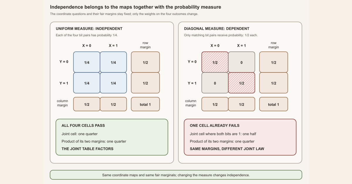
Take two fair coins, or equivalently two fair bits. The first bit will be called \(X\), and the second will be called \(Y\). There are four possible outcomes:
\[ \Omega=\{(0,0),(0,1),(1,0),(1,1)\}. \]The set \(\Omega\) is the sample space, the complete list of outcomes in this finite model. Put the uniform probability measure \(\mathbb P_{\mathrm u}\) on it:
\[ \mathbb P_{\mathrm u}\{\omega\}=\frac14 \qquad\text{for every }\omega\in\Omega. \]Define the two coordinate readouts by
\[ X(a,b)=a, \qquad Y(a,b)=b. \]These are random variables : measurable functions from outcomes to values. In this finite model every subset is declared measurable, so no event is hidden from the probability measure.
Compute the complete joint table
The joint probability in a cell records both readouts at once. A marginal probability ignores one coordinate and sums across its row or column.
| Under \(\mathbb P_{\mathrm u}\) | \(X=0\) | \(X=1\) | Row margin |
|---|---|---|---|
| \(Y=0\) | \(1/4\) | \(1/4\) | \(\mathbb P_{\mathrm u}\{Y=0\}=1/2\) |
| \(Y=1\) | \(1/4\) | \(1/4\) | \(\mathbb P_{\mathrm u}\{Y=1\}=1/2\) |
| Column margin | \(\mathbb P_{\mathrm u}\{X=0\}=1/2\) | \(\mathbb P_{\mathrm u}\{X=1\}=1/2\) | \(1\) |
For the upper-right cell, for example,
\[ \begin{aligned} \mathbb P_{\mathrm u}\{X=1,\ Y=0\} &=\frac14,\\ \mathbb P_{\mathrm u}\{X=1\}\, \mathbb P_{\mathrm u}\{Y=0\} &=\frac12\cdot\frac12 =\frac14. \end{aligned} \]The same calculation works for all four cells. Because the target \(\{0,1\}\) has only four subsets and each is a union of singleton values, checking these four singleton cells is enough in this particular finite example. It would not be enough to check only a few convenient values in a general measurable space.
Thus \(X\) and \(Y\) are independent under \(\mathbb P_{\mathrm u}\).
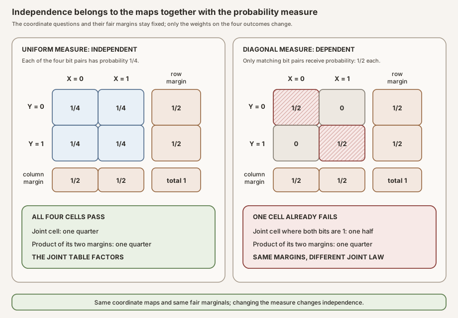
The same maps become dependent under another measure
Keep the same sample space and the same coordinate functions \(X\) and \(Y\). Change only the probability measure:
\[ \mathbb P_{\mathrm d}\{(0,0)\} =\mathbb P_{\mathrm d}\{(1,1)\} =\frac12, \]while
\[ \mathbb P_{\mathrm d}\{(0,1)\} =\mathbb P_{\mathrm d}\{(1,0)\} =0. \]The subscript \(\mathrm d\) stands for diagonal, because all probability mass lies on the diagonal cells of the table. Both margins are still fair:
\[ \mathbb P_{\mathrm d}\{X=1\} =\mathbb P_{\mathrm d}\{Y=1\} =\frac12. \]But their joint event fails the product test:
\[ \mathbb P_{\mathrm d}\{X=1,\ Y=1\} =\frac12 \ne \frac12\cdot\frac12 =\mathbb P_{\mathrm d}\{X=1\} \,\mathbb P_{\mathrm d}\{Y=1\}. \]Under \(\mathbb P_{\mathrm d}\), learning \(X\) tells us \(Y\) exactly. The variables are dependent even though each variable, viewed alone, still looks like a fair bit.
This comparison isolates the dependence on the probability measure:
Independence is a property of the functions together with the chosen probability measure. It is not a property of their formulas alone.
Equal marginal laws also do not determine a joint law. Both models have the same two fair marginals, but one joint table is uniform and the other is concentrated on two cells.
The general definition
Let \(\Omega\) be a sample space equipped with a probability measure \(\mathbb P\). Let \(S\) and \(T\) be measurable target spaces, and let
\[ X:\Omega\longrightarrow S, \qquad Y:\Omega\longrightarrow T \]be measurable random variables. For target sets \(A\subseteq S\) and \(B\subseteq T\), the preimages
\[ X^{-1}(A)=\{\omega:X(\omega)\in A\}, \qquad Y^{-1}(B)=\{\omega:Y(\omega)\in B\} \]are source events .
The variables \(X\) and \(Y\) are independent under \(\mathbb P\) when
\[ \begin{aligned} \mathbb P\!\left(X^{-1}(A)\cap Y^{-1}(B)\right) &= \mathbb P\!\left(X^{-1}(A)\right)\, \mathbb P\!\left(Y^{-1}(B)\right). \end{aligned} \]for every measurable target set \(A\) and every measurable target set \(B\). The words “for every” do real work. One successful cell or one zero-probability coincidence does not establish independence.
The informal phrase “learning \(X\) does not change the probability of \(Y\)” comes from conditional probability. When \(\mathbb P(X\in A)\gt0\), factorization is equivalent to
\[ \mathbb P(Y\in B\mid X\in A)=\mathbb P(Y\in B). \]The factorization definition is more fundamental because it remains meaningful when the conditioning event has probability zero.
The same statement at the level of laws
The joint probability law of \((X,Y)\) assigns probabilities to sets of pairs. The two marginal laws assign probabilities to values of \(X\) and \(Y\) separately. Independence is equivalent, under the standard measurability hypotheses, to
\[ \begin{aligned} \mathcal L_{\mathbb P}(X,Y) &= \mathcal L_{\mathbb P}(X)\otimes \mathcal L_{\mathbb P}(Y). \end{aligned} \]The symbol \(\otimes\) denotes the product of measures here, not a tensor product of vectors. This equality says that the complete joint law is fixed by multiplying the marginal laws. Without independence, the marginals leave the coupling between coordinates undetermined, exactly as the two bit tables show.
Pairwise independence is not mutual independence
For an indexed family \((X_i)_{i\in I}\), mutual independence means that every finite collection of measurable coordinate events factors. If \(J\subseteq I\) is finite and each \(A_j\) is measurable, then
\[ \begin{aligned} \mathbb P\!\left( \bigcap_{j\in J}\{X_j\in A_j\} \right) &= \prod_{j\in J}\mathbb P\{X_j\in A_j\}. \end{aligned} \]Pairwise independence checks only pairs of distinct indices. It is weaker. Here is an exact four-outcome counterexample.
Take independent fair bits \(U\) and \(V\), and define
\[ W=U\mathbin{\mathsf{xor}}V, \]where exclusive-or, written \(\mathsf{xor}\), is addition modulo \(2\). The four equally likely triples are
| \(U\) | \(V\) | \(W=U\mathbin{\mathsf{xor}}V\) | Probability |
|---|---|---|---|
| \(0\) | \(0\) | \(0\) | \(1/4\) |
| \(0\) | \(1\) | \(1\) | \(1/4\) |
| \(1\) | \(0\) | \(1\) | \(1/4\) |
| \(1\) | \(1\) | \(0\) | \(1/4\) |
For any pair among \(U,V,W\), the four possible pair values occur exactly once, so each pair is independent. The triple is not mutually independent:
\[ \mathbb P\{U=0,V=0,W=0\} =\frac14, \]but the product of the three marginal probabilities is
\[ \mathbb P\{U=0\}\, \mathbb P\{V=0\}\, \mathbb P\{W=0\} =\frac12\cdot\frac12\cdot\frac12 =\frac18. \]The deterministic relation \(W=U\mathbin{\mathsf{xor}}V\) becomes visible only when all three coordinates are considered together. The project’s finite Gaussian families use mutual independence, not merely pairwise independence, because a full product law is a statement about the entire family.
Independence is not identical distribution
The phrase independent and identically distributed (i.i.d.) combines two separate properties:
- independent says how the joint law factors;
- identically distributed says all one-coordinate marginal laws are equal.
Variables can be independent while having different means, variances, or even different target spaces. Conversely, the diagonal bit example has identical fair marginals but dependence.
Independence is also stronger than zero covariance in general. For real random variables with finite second moments, the covariance is
\[ \begin{aligned} \operatorname{Cov}_{\mathbb P}(X,Y) &= \mathbb E_{\mathbb P} \!\left[ \bigl(X-\mathbb E_{\mathbb P}[X]\bigr) \bigl(Y-\mathbb E_{\mathbb P}[Y]\bigr) \right]. \end{aligned} \]Independence implies zero covariance under these moment assumptions. The converse can fail. For example, let \(Z\) be uniform on \(\{-1,0,1\}\) and set \(Q=Z^2\). Then \(Q\) is determined by \(Z\), so the pair is dependent, while symmetry gives \(\mathbb E[Z]=\mathbb E[Z^3]=0\), hence \(\operatorname{Cov}(Z,Q)=0\).
For jointly Gaussian variables, zero covariance does characterize independence. The word jointly is essential: Gaussian marginal laws alone do not supply a joint Gaussian law.
Gaussian coordinates and variance addition
Independence makes coordinatewise probability models assemble cleanly. If a finite family \(X_i\) is mutually independent and coordinate \(i\) has Gaussian law
\[ X_i\sim\mathcal N(m_i,v_i), \]then the joint law is the product of those coordinate laws:
\[ \begin{aligned} \mathcal L\bigl((X_i)_{i\in I}\bigr) &= \bigotimes_{i\in I}\mathcal N(m_i,v_i). \end{aligned} \]This is the bridge used by the project to build exact finite Gaussian coordinate spaces. It separates three obligations:
- each coordinate map is measurable;
- each coordinate has its stated Gaussian law; and
- the entire family is mutually independent under the named measure.
Coordinatewise deterministic transformations preserve independence when the
transformations are measurable. In particular, scaling coordinate \(i\) by a
constant does not mix information from different coordinates. The project’s
IndependentRealGaussianFamily.scale theorem uses this fact while
updating the mean and variance parameters.
For two independent real variables with finite second moments,
\[ \begin{aligned} \operatorname{Var}_{\mathbb P}(X+Y) &= \operatorname{Var}_{\mathbb P}(X) {}+ \operatorname{Var}_{\mathbb P}(Y). \end{aligned} \]The missing cross term is twice the covariance, which vanishes under independence. If the variables also have exact Gaussian laws \(\mathcal N(m_X,v_X)\) and \(\mathcal N(m_Y,v_Y)\), then their sum has the exact law
\[ X+Y\sim\mathcal N(m_X+m_Y,\ v_X+v_Y). \]The project theorem HasRealGaussianLaw.add_of_indep records this
law-level conclusion. Variance addition is a consequence here, not a general
test for independence: dependent variables can sometimes have zero covariance
and the same variance identity.
These distinctions matter when setting a normalization convention for random matrices. Choosing the variance of each free coordinate and proving their mutual independence are separate tasks.
In Lean
Mathlib names independence of two functions IndepFun. The measure
is an explicit argument, so the type records the dependence exposed by the two
bit tables.
ProbabilityTheory.IndepFun X Y PXandYare functions with a common source typeΩ. Their target types may differ.P : Measure Ωis the measure used in every probability. ChangingPcan change whether the same functions are independent.ProbabilityTheory.IndepFunis the fully qualified predicate. Withopen scoped ProbabilityTheory, Lean also acceptsX ⟂ᵢ[P] Y.- The subscript-like symbol in
⟂ᵢis part of Mathlib’s notation for independence. The bracketed[P]names the measure; it is not an implicit default. - Measurable spaces on the source and targets tell Lean which sets count as measurable questions. They are typeclass arguments carried by the context.
The pinned Mathlib theorem below is the exact preimage-factorization interface
behind the paper definition. Its ambient variables are functions
f and g on the same source and a measure
μ.
theorem indepFun_iff_measure_inter_preimage_eq_mul {mβ : MeasurableSpace β}
    {mβ' : MeasurableSpace β'} :
    f ⟂ᵢ[μ] g ↔
      ∀ s t, MeasurableSet s → MeasurableSet t
        → μ (f ⁻¹' s ∩ g ⁻¹' t) = μ (f ⁻¹' s) * μ (g ⁻¹' t) := by
  simp only [IndepFun, Kernel.indepFun_iff_measure_inter_preimage_eq_mul,
    ae_dirac_eq, Filter.eventually_pure, Kernel.const_apply]
Read ↔ as “if and only if,” ∀ s t as “for every
target set s and t,” and
f ⁻¹’ s as the preimage of s under
f. The symbol ∩ is event intersection, and
μ (…) asks the measure for that event’s mass. The final
* multiplies two nonnegative extended-real measure values.
For a family, Mathlib uses iIndepFun X P. Its finite-event
interface multiplies over a Finset, a finite set of indices:
theorem iIndepFun_iff_measure_inter_preimage_eq_mul {ι : Type*} {β : ι → Type*}
    {m : ∀ x, MeasurableSpace (β x)} {f : ∀ i, Ω → β i} :
    iIndepFun f μ ↔
      ∀ (S : Finset ι) {sets : ∀ i : ι, Set (β i)}
        (_H : ∀ i, i ∈ S → MeasurableSet[m i] (sets i)),
        μ (⋂ i ∈ S, f i ⁻¹' sets i) =
          ∏ i ∈ S, μ (f i ⁻¹' sets i) := by
  simp only [iIndepFun, Kernel.iIndepFun_iff_measure_inter_preimage_eq_mul,
    ae_dirac_eq, Filter.eventually_pure, Kernel.const_apply]
The displayed declaration is reformatted from the exact pinned source without
changing its statement or proof. The empty finite set is among the cases
encoded by iIndepFun; Mathlib consequently derives that its base
measure is a probability measure.
A tiny standalone worksheet
The following Lean program checks the two tables without Mathlib. A row’s
natural-number weight is measured in quarter-units, so both
tables have total weight \(4\). The identity
is exactly the denominator-cleared probability factorization.
Save this complete block as IndependenceWorksheet.lean:
import Std

structure WeightedOutcome where
  x : Bool
  y : Bool
  weight : Nat
deriving Repr

def uniformRows : List WeightedOutcome :=
  [ { x := false, y := false, weight := 1 }
  , { x := false, y := true,  weight := 1 }
  , { x := true,  y := false, weight := 1 }
  , { x := true,  y := true,  weight := 1 } ]

def diagonalRows : List WeightedOutcome :=
  [ { x := false, y := false, weight := 2 }
  , { x := false, y := true,  weight := 0 }
  , { x := true,  y := false, weight := 0 }
  , { x := true,  y := true,  weight := 2 } ]

def massWhere (rows : List WeightedOutcome)
    (p : WeightedOutcome → Bool) : Nat :=
  rows.foldl
    (fun total row =>
      match p row with
      | true => total + row.weight
      | false => total)
    0

def totalWeight (rows : List WeightedOutcome) : Nat :=
  massWhere rows (fun _ => true)

def jointWeight (rows : List WeightedOutcome) (x y : Bool) : Nat :=
  massWhere rows (fun row => (row.x == x) && (row.y == y))

def xMarginWeight (rows : List WeightedOutcome) (x : Bool) : Nat :=
  massWhere rows (fun row => row.x == x)

def yMarginWeight (rows : List WeightedOutcome) (y : Bool) : Nat :=
  massWhere rows (fun row => row.y == y)

def factorsAt (rows : List WeightedOutcome) (x y : Bool) : Bool :=
  jointWeight rows x y * totalWeight rows ==
    xMarginWeight rows x * yMarginWeight rows y

def bitValues : List Bool := [false, true]

def independentBits (rows : List WeightedOutcome) : Bool :=
  bitValues.all fun x =>
    bitValues.all fun y =>
      factorsAt rows x y

#eval independentBits uniformRows
#eval independentBits diagonalRows

example : independentBits uniformRows = true := by decide
example : independentBits diagonalRows = false := by decide
On an ordinary Mac or Linux machine with Elan and the pinned Lean toolchain already installed, a human types:
elan run leanprover/lean4:v4.32.0 lean IndependenceWorksheet.lean
Lean prints true for the uniform table and false for
the diagonal table. The two example declarations then ask the
kernel to certify those computations. This miniature uses finite integer
weights and binary singleton checks. It does not define Mathlib measures or
prove ProbabilityTheory.IndepFun.
The checked project layer
The project bundles measurability, exact Gaussian coordinate laws, and mutual independence as separate fields:
structure IndependentRealGaussianFamily (X : ι → Ω → ℝ) (m : ι → ℝ)
    (v : ι → ℝ≥0) (P : Measure Ω) : Prop where
  measurable : ∀ i, Measurable (X i)
  hasLaw : ∀ i, HasRealGaussianLaw (X i) (m i) (v i) P
  independent : iIndepFun X P
For a finite index type, the project’s exact theorem turns those coordinate facts into the joint product law:
theorem jointHasLaw (hX : IndependentRealGaussianFamily X m v P) :
    HasLaw (fun ω i ↦ X i ω)
      (Measure.pi fun i ↦ gaussianReal (m i) (v i)) P :=
  hX.independent.hasLaw_pi hX.hasLaw
The two-variable Gaussian sum theorem keeps the independence hypothesis visible:
theorem add_of_indep (hX : HasRealGaussianLaw X mX vX P)
    (hY : HasRealGaussianLaw Y mY vY P) (hXY : IndepFun X Y P) :
    HasRealGaussianLaw (fun ω ↦ X ω + Y ω) (mX + mY) (vX + vY) P := by
  simpa only [HasRealGaussianLaw, gaussianReal_conv_gaussianReal] using
    hXY.hasLaw_fun_add hX hY
The authoritative project source is
formalization/NonlinearDynamics/Random/GaussianPrimitives.lean.
A learner can put these lines in a temporary scratch file inside the
formalization project. This full project check uses the
repository’s pinned Lean and Mathlib dependencies:
import NonlinearDynamics.Random.GaussianPrimitives

open MeasureTheory ProbabilityTheory
open scoped ProbabilityTheory

#check ProbabilityTheory.IndepFun
#check ProbabilityTheory.indepFun_iff_measure_inter_preimage_eq_mul
#check ProbabilityTheory.iIndepFun
#check ProbabilityTheory.iIndepFun.hasLaw_pi
#check ProbabilityTheory.IndepFun.variance_add
#check NonlinearDynamics.Random.HasRealGaussianLaw.add_of_indep
#check NonlinearDynamics.Random.IndependentRealGaussianFamily
#check NonlinearDynamics.Random.IndependentRealGaussianFamily.jointHasLaw
#check NonlinearDynamics.Random.gaussianProductMeasure_iIndepFun
import loads the checked project module and its pinned Mathlib
dependencies. Each #check asks Lean to elaborate the named
declaration and report its type; it does not create a new theorem. The literal
full-project command below checks the authoritative project file itself.
cd formalization
lake env lean -DwarningAsError=true NonlinearDynamics/Random/GaussianPrimitives.lean
Resource note: this exact file uses the repository's
pinned Lean and Mathlib dependencies. Initial project setup can require
substantial disk space and build time. For a lightweight first step on
macOS or Linux, use the page's standalone Lean-core or Std
tutorial.
Distinctions and boundary cases
| Do not confuse | With | Why the difference matters |
|---|---|---|
| Independent variables | Variables with equal marginal laws | The diagonal table has two fair marginals but dependence |
| Pairwise independence | Mutual independence | The \(U,V,U\mathbin{\mathsf{xor}}V\) family passes every pair check but fails a triple check |
| Zero covariance | Independence | \(Z\) and \(Z^2\) can have zero covariance while one determines the other |
| Gaussian marginals | A jointly Gaussian vector | Separate one-variable laws do not determine the coupling |
| A function formula | Independence under a measure | The same coordinate maps are independent under \(\mathbb P_{\mathrm u}\) and dependent under \(\mathbb P_{\mathrm d}\) |
| Independence | Causal separation | A factorized law is a probabilistic property, not by itself a claim about physical causes |
| Product law | Tensor product of vectors | The product here combines measures on coordinate spaces |
Constant random variables can be independent: degeneracy alone does not create dependence. Coordinatewise measurable transformations preserve independence, but a transformation that mixes several coordinates can create new dependencies among the outputs. Independence also does not imply identical distribution.
Where to continue
The probability measure page explains the object that assigns the cell masses. The random variable page separates a sample map from its law . The variance page develops the scale parameter that adds for independent sums.
The Gaussian distribution page defines each coordinate law, while the normalization convention page explains what must be fixed before scaling those coordinates. The Deep Dive Gaussian Laws, Independence, and Normalization shows how finite product measures and exact Lean laws fit together.
Complex Gaussian Coordinates and Geometry turns one independent real pair into an exact complex law. The Independent Cartesian complex Gaussian family page then scales mutual independence across indexed complex blocks. Finally, Finite Product Probability Spaces and Independent Gaussian Fields explains why pairwise independence, within-pair independence, and separate source families do not replace one exact field product law.
References
Mathlib contributors.
Independence of functions,
Mathlib 4 documentation. This official implementation reference defines
IndepFun and iIndepFun and states their measurable
event factorization theorems.
Mathlib contributors.
Law of a random variable,
Mathlib 4 documentation. The theorem iIndepFun.hasLaw_pi turns
mutual independence plus coordinate laws into a joint
Measure.pi law.
Mathlib contributors.
Variance of random variables,
Mathlib 4 documentation. This official source includes
IndepFun.variance_add with its finite-second-moment hypotheses.
Olav Kallenberg. Foundations of Modern Probability, third edition, Springer, 2021. This is a standard reference for independence, product laws, and finite-dimensional distributions.
The local code uses the exact Mathlib 4.32.0 dependency pinned at commit 81a5d257.