Independent Cartesian complex Gaussian family

Start with two complex coordinates

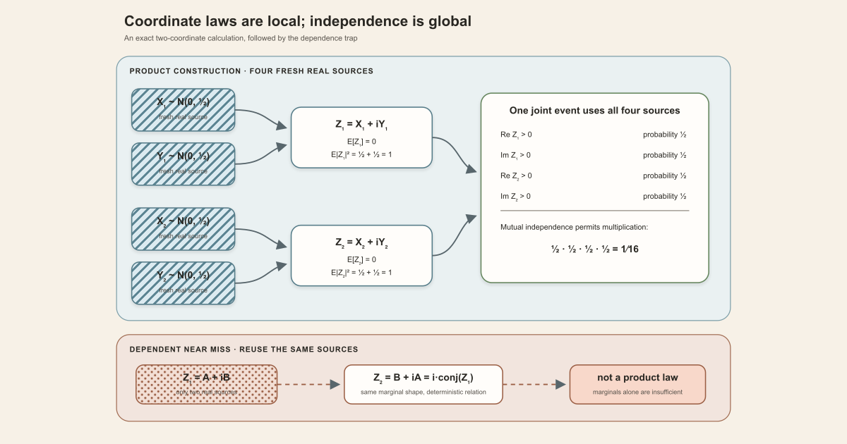
Take four mutually independent real Gaussian variables

and combine them in pairs:

Each complex coordinate has mean zero and total centered squared magnitude

The family statement adds more than these two marginal calculations. Because all four real sources are mutually independent, the two complex blocks are independent. Symmetry gives a checkable event calculation: each component is positive with probability \(1/2\), so

If instead \(Z_2=i\overline{Z_1}\), both coordinates still have the same centered Cartesian Gaussian marginal law, but the second is determined by the first. The joint law is then not a product. Correct coordinate laws are not a substitute for family independence.

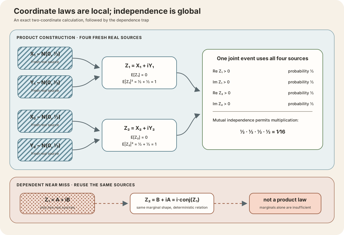
An independent Cartesian complex Gaussian family is an indexed collection of complex-valued random variables in which every coordinate has a named exact Cartesian complex Gaussian law and all complex coordinates are mutually independent. The word Cartesian keeps the real-part and imaginary-part variances visible. The word independent applies across the indexed complex variables, not only inside one real-imaginary pair.

Let \(\iota\) be an index type, let \((\Omega,\mathcal F,P)\) be a measured space, and write

For each index, choose a complex mean \(m_i\) and nonnegative coordinate variances \(v_{\mathrm R,i}\) and \(v_{\mathrm I,i}\). The project bundle records three different obligations:

1. every map \(Z_i\) is ordinarily measurable;
2. every \(Z_i\) has the exact Cartesian law with parameters \((m_i,v_{\mathrm R,i},v_{\mathrm I,i})\); and
3. the family \((Z_i)_{i\in\iota}\) is mutually independent under \(P\).

The exact project definition

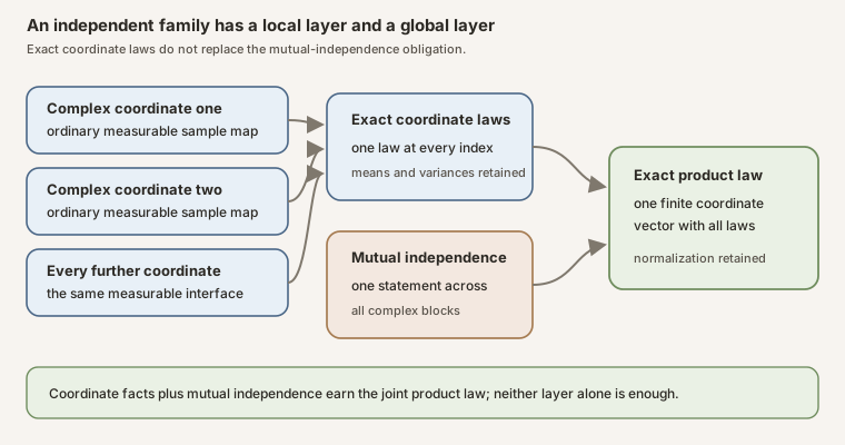
IndependentCartesianComplexGaussianFamily Z m vRe vIm P

In Lean, the structure is parameterized by four functions and a base measure:

structure IndependentCartesianComplexGaussianFamily
    (Z : ι → Ω → ℂ) (m : ι → ℂ) (vRe vIm : ι → ℝ≥0)
    (P : Measure Ω) : Prop where
  measurable : ∀ i, Measurable (Z i)
  hasLaw : ∀ i,
    HasCartesianComplexGaussianLaw (Z i) (m i) (vRe i) (vIm i) P
  independent : iIndepFun Z P

iIndepFun is Mathlib’s indexed mutual-independence predicate for functions. It is stronger than listing independence for a few selected pairs. The structure keeps it separate from the coordinate laws because a collection of correct marginals does not determine a joint law.

The ordinary Measurable field is also deliberate. The exact probability law predicate HasLaw carries almost-everywhere measurability, which ignores changes on null sets. Later coordinatewise constructions benefit from an ordinary measurable map at each index, so the family stores that stronger fact because it cannot be recovered from equality in law.

Three independence questions, not one

For one variable \(Z_i=X_i+iY_i\), its Cartesian law says that \(X_i\) and \(Y_i\) are independent real Gaussians. That is within-coordinate independence.

For distinct indices, mutual independence of the complex maps says that the blocks \(Z_i\) are independent. That is between-coordinate independence. Together with the exact Cartesian laws, this yields the fully factored finite joint law.

A third question appears when a construction begins from one real family \((X_i)\) and another real family \((Y_i)\): are the two families independent of each other? Separate mutual independence inside the \(X\)-family and inside the \(Y\)-family does not answer that cross-family question.

A two-index counterexample makes the gap visible. Let \(A\) and \(B\) be independent standard real Gaussians, and set

The \(X\)-family is independent, the \(Y\)-family is independent, and each pair \((X_i,Y_i)\) has independent coordinates. Yet

The two complex variables are deterministically related, so they are not independent. The checked constructor therefore asks for mutually independent pair-vectors \((X_i,Y_i)\), each with the exact product law. It never infers a missing cross-family hypothesis.

Type a finite independence skeleton locally

The continuous Gaussian proof belongs to Mathlib and the project. A much smaller Std-only worksheet lets a beginner check the combinatorial factorization behind the \(1/16\) calculation. Save this as FourIndependentSigns.lean outside the project:

import Std

structure FourSigns where
  x1Positive : Bool
  y1Positive : Bool
  x2Positive : Bool
  y2Positive : Bool
deriving Repr, DecidableEq

def signs : List Bool := [false, true]

def outcomes : List FourSigns :=
  signs.flatMap fun x1 =>
  signs.flatMap fun y1 =>
  signs.flatMap fun x2 =>
  signs.map fun y2 =>
    { x1Positive := x1, y1Positive := y1,
      x2Positive := x2, y2Positive := y2 }

def firstQuadrantZ1 (ω : FourSigns) : Bool :=
  ω.x1Positive && ω.y1Positive

def bothFirstQuadrants (ω : FourSigns) : Bool :=
  firstQuadrantZ1 ω && ω.x2Positive && ω.y2Positive

#eval outcomes.length
#eval (outcomes.filter firstQuadrantZ1).length
#eval (outcomes.filter bothFirstQuadrants).length

example : outcomes.length = 16 := by decide
example : (outcomes.filter firstQuadrantZ1).length = 4 := by decide
example : (outcomes.filter bothFirstQuadrants).length = 1 := by decide

Run the file with the already-installed pinned compiler:

elan run leanprover/lean4:v4.32.0 lean FourIndependentSigns.lean

Lean prints \(16\), \(4\), and \(1\). Under the uniform law on the sixteen rows, the first complex coordinate lands in its first quadrant with probability \(4/16=1/4\), and both do so with probability \(1/16\). The worksheet models four independent signs, not Gaussian magnitudes; it isolates the finite factorization step and does not formalize continuous probability with a list.

Finite families have an exact product joint law

When \(\iota\) is finite, collect all coordinates into one sample map

The theorem IndependentCartesianComplexGaussianFamily.jointHasLaw identifies its exact law:

In Lean the right side is Measure.pi. This is stronger than knowing the coordinate means, variances, or even all pairwise laws. It fixes the probability of every measurable event in the finite function space.

The neighboring theorem jointHasGaussianLaw omits the explicit parameters and retains qualitative Gaussianity on the finite real vector space \(\iota\to\mathbb C\). The exact product theorem should remain the primary statement whenever normalization data matters.

A three-coordinate worked ledger

Take a three-element index type with labels a, b, and c. The following symbolic ledger illustrates what the four parameter functions can store:

Coordinate a has equal component variances, but the family structure does not attach a circularity theorem to that numerical coincidence. Coordinate b is anisotropic. Coordinate c has a zero real-part variance, so its law is supported on a vertical line through its mean. All three cases fit one family type.

If the three complex coordinates are mutually independent, their field law is the product of these three exact measures. Replacing the variance table with a different schedule changes that product law without changing the family interface. This is why vRe and vIm remain functions rather than one global scale.

The marginal table alone is insufficient for a product-law conclusion. One could construct three variables with exactly these marginal parameters while reusing hidden source randomness across indices. The independent field is the additional evidence that turns the coordinate ledger into an exact joint measure. These values are a teaching example, not an empirical result or a selected matrix convention.

Why the exact law matters beyond moments

Means and variances cannot identify a probability law in general. Even within a Gaussian discussion, a list of coordinate laws does not identify their coupling. The exact HasLaw statement for the complete field answers every measurable question about the coordinate vector, not only questions built from first and second moments.

For example, it determines probabilities of simultaneous coordinate events and expectations of bounded measurable functions of the whole field. The project can therefore move the family through a later measurable matrix assembly map and obtain an exact matrix pushforward law. A parameter table without the joint measure would not support that transport.

Real scaling preserves the family interface

A real scale \(c_i\) acts coordinatewise by

The mean becomes \(c_i m_i\), and both Cartesian variances acquire the same squared factor:

The theorem scale preserves ordinary measurability, every exact coordinate law, and mutual independence. Negative scales reflect both axes, while a zero scale produces the correct Dirac coordinate. A general complex scale can mix the displayed real and imaginary axes, so this theorem intentionally accepts real scales only.

The canonical product realization

For a finite index type, the measure cartesianComplexGaussianProductMeasure m vRe vIm lives directly on the function space \(\iota\to\mathbb C\). Its sample point is already a complete coordinate assignment. Evaluation at index \(i\),

has the requested exact Cartesian law, and the evaluation maps are mutually independent. The theorem cartesianComplexGaussianProductMeasure_independentFamily bundles those facts into the same family interface.

This canonical space is a convenient witness, not the only possible outcome space. Any family on another space with the same exact joint law is distributionally equivalent for measurable questions about the coordinate vector.

If \(\iota\) is empty, the function space \(\iota\to\mathbb C\) contains one function. The empty product law is therefore the Dirac measure at that unique empty assignment. The checked theorem cartesianComplexGaussianProductMeasure_eq_dirac_of_isEmpty states exactly this boundary. It does not decide what a zero-dimensional matrix ensemble should mean.

Checked consequences and explicit nonclaims

Inspect the exact project interface

In a clone with the repository’s pinned Lean and Mathlib dependencies installed, a human can type:

import NonlinearDynamics.Random.ComplexGaussianFamilies

#print NonlinearDynamics.Random.IndependentCartesianComplexGaussianFamily
#check NonlinearDynamics.Random.IndependentCartesianComplexGaussianFamily.jointHasLaw
#check NonlinearDynamics.Random.IndependentCartesianComplexGaussianFamily.jointHasGaussianLaw
#check NonlinearDynamics.Random.IndependentCartesianComplexGaussianFamily.scale
#check NonlinearDynamics.Random.cartesianComplexGaussianProductMeasure_independentFamily
#check NonlinearDynamics.Random.cartesianComplexGaussianProductMeasure_eq_dirac_of_isEmpty

#print exposes the complete structure rather than only its name. The first two #check lines distinguish the exact product law from the qualitative Gaussian consequence. The remaining checks inspect scaling, the canonical finite product witness, and the empty-index boundary.

cd formalization
lake env lean -DwarningAsError=true NonlinearDynamics/Random/ComplexGaussianFamilies.lean

The Lean module exposes each coordinate’s exact real and imaginary laws, means, variances, finite-exponent MemLp, and integrability. It also checks real scaling, construction from independent pair-vectors, the finite product joint law, the canonical sample space, and the empty-index Dirac identity.

It does not establish any of the following:

• pairwise independence as a replacement for mutual independence;
• cross-family independence from two separately independent real families;
• equal real and imaginary variances;
• circular symmetry, properness, or a planar density;
• a dimension-dependent matrix normalization;
• a Gaussian unitary ensemble (GUE) law within this module;
• independence of every entry of a Hermitian matrix, whose lower triangle is determined by conjugate reflection; or
• unitary invariance, eigenvalue laws, trace moments, or asymptotics.

Where to continue

Read independence for event factorization and the difference between pairwise and mutual claims. The Cartesian complex Gaussian law entry develops the single-coordinate law, while normalization convention explains why the two variance functions must remain visible.

The Deep Dive Finite Product Probability Spaces and Independent Gaussian Fields develops the product-space construction, dependence audit, empty boundary, and future matrix bridge in full.

The next deterministic bridge is the Hermitian coordinate space . Finite Hermitian Matrices from Coordinates shows how complex strict-upper coordinates enter a Hermitian matrix without claiming that this family supplies the real diagonal or fixes a Gaussian matrix normalization.

Finite GUE from Independent Gaussian Coordinates then supplies the real diagonal block, selects the Wigner variances, joins both blocks under one product measure, and transports them to the matrix law.

References

Mathlib contributors. Independence of functions, Mathlib 4 documentation. This is the official API for IndepFun, iIndepFun, measurable coordinate transformations, and finite joint product laws.

Mathlib contributors. Finite product measures, Mathlib 4 documentation. This is the official source for Measure.pi, coordinate evaluation, probability preservation, and the empty product.

N. R. Goodman. Statistical Analysis Based on a Certain Multivariate Complex Gaussian Distribution (An Introduction), The Annals of Mathematical Statistics 34(1), 152-177, 1963. This original article supplies historical context for complex multivariate Gaussian laws; it does not choose this project’s normalization.

The exact upstream Lean source audited for this entry is Mathlib commit 81a5d257, the revision pinned by this repository.