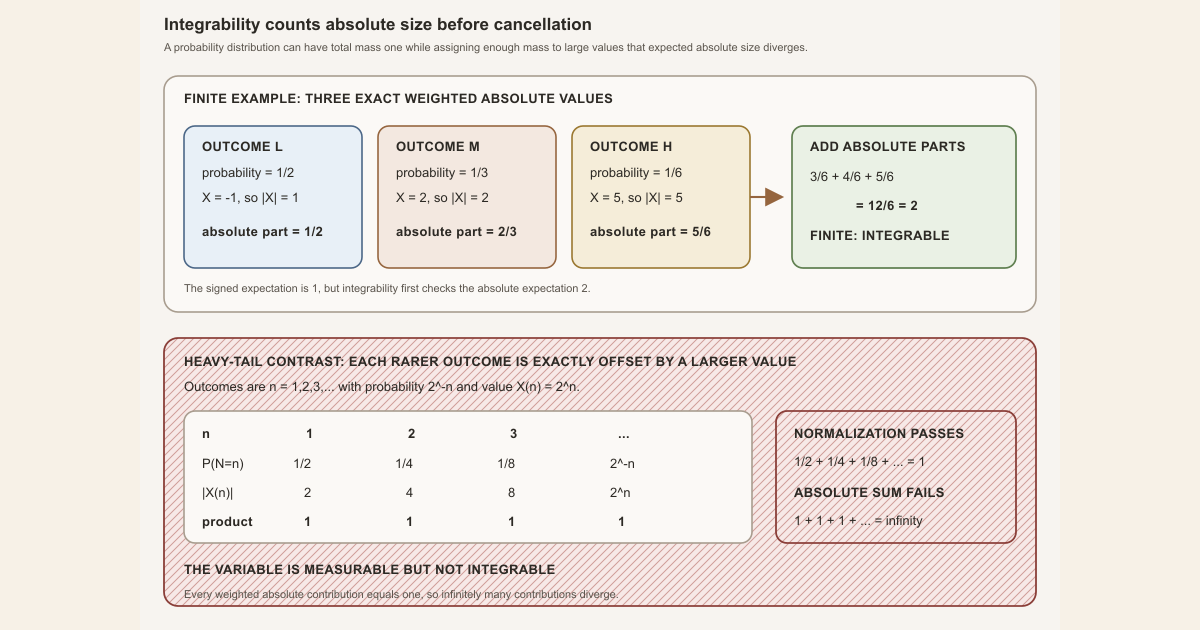
An integrable real-valued function has finite total absolute size under a chosen measure. On a space with a probability measure , this means
\[ \mathbb E_\mu[|X|] {} = \int_\Omega |X(\omega)|\,d\mu(\omega) \lt\infty. \]Absolute integrability is the relevant condition. Positive and negative contributions cannot hide infinite absolute size by cancellation.
Start with three exact outcomes
Let
\[ \Omega=\{L,M,H\} \]and assign probabilities
\[ \mu\{L\}=\frac12, \qquad \mu\{M\}=\frac13, \qquad \mu\{H\}=\frac16. \]They form a probability measure because
\[ \frac12+\frac13+\frac16 {} = \frac36+\frac26+\frac16 {} = 1. \]Define a payoff \(X\) by
\[ X(L)=-1, \qquad X(M)=2, \qquad X(H)=5. \]On this finite discrete space, \(X\) is measurable. Its expected absolute size is
\[ \begin{aligned} \mathbb E_\mu[|X|] &=\frac12|-1|+\frac13|2|+\frac16|5|\\ &=\frac12+\frac23+\frac56\\ &=\frac36+\frac46+\frac56\\ &=\frac{12}{6}\\ &=2. \end{aligned} \]Because \(2\lt\infty\), \(X\) is integrable. Its signed expectation is
\[ \mathbb E_\mu[X] {} = -\frac12+\frac23+\frac56 {} = 1. \]The two numbers answer different questions. The value \(2\) certifies finite absolute size. The value \(1\) is the probability-weighted signed average.
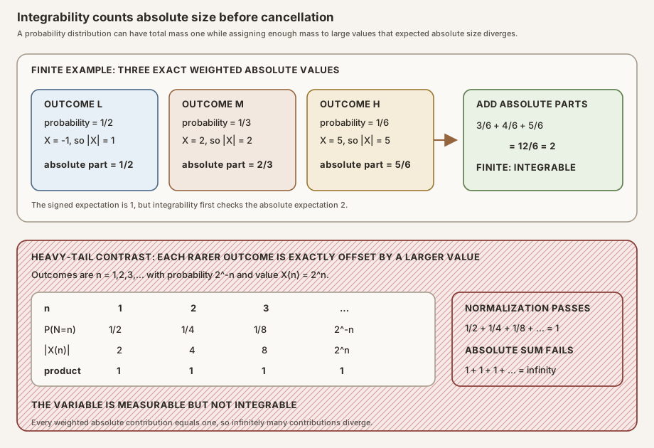
A normalized heavy tail that is not integrable
Now let the outcomes be the positive integers
\[ \Omega=\{1,2,3,\ldots\}, \]with every subset measurable. Define
\[ \mathbb P\{N=n\}=2^{-n} \qquad\text{for }n\ge1. \]Here \(2^{-n}=1/2^n\). The indexing starts at one, so the total probability is
\[ \sum_{n=1}^{\infty}2^{-n} {} = \frac{1/2}{1-1/2} {} = 1. \]Thus the distribution is normalized exactly; no mass is missing.
Define the nonnegative random variable
\[ X(n)=2^n. \]It is measurable because the source and target use their usual discrete and Borel measurable structures. Every individual value is finite. Nevertheless,
\[ \begin{aligned} \mathbb E[|X|] &=\sum_{n=1}^{\infty}|2^n|\,2^{-n}\\ &=\sum_{n=1}^{\infty}1\\ &=\infty. \end{aligned} \]So \(X\) is not integrable. The probabilities become small, but the values grow at exactly the reciprocal rate. Every outcome level contributes one unit to the absolute expectation, and infinitely many unit contributions diverge.
Because \(X\ge0\), probability texts may write
\(\mathbb E[X]=\infty\) as an extended expectation. That is not a finite
real expectation, and it does not satisfy the project’s
Integrable X μ gate.
The four layers to keep separate
Let \(f:\Omega\to\mathbb R\) and let \(\mu\) be a measure on \(\Omega\).
| Layer | Question | Mathematical form |
|---|---|---|
| Measurability | Are inverse images of measurable value sets measurable source events? | \(f\) is measurable |
| Finite absolute integral | Is the total norm finite? | (\int_\Omega |
| Integrability | Do the regularity and finite-size gates both hold? | \(f\in L^1(\mu)\) |
| Expectation | What signed average does an integrable variable have under probability mass one? | \(\mathbb E_\mu[f]=\int_\Omega f\,d\mu\) |
The measurability condition is about admissible preimages. It supplies no finite bound. The heavy-tail \(X\) is the concrete counterexample: measurable, but not integrable.
For real-valued functions, absolute integrability means exactly that the integral of \(|f|\) is finite. This is the size component of Lebesgue or Bochner integrability. Merely obtaining a finite answer from a conditionally convergent signed series is not enough. For example, the alternating harmonic series converges as an ordered series, but its absolute series diverges; it does not define an integrable function under counting measure.
Once \(\mathbb E[|X|]\lt\infty\), both the positive and negative parts have finite mass, so the signed expectation is a finite real number rather than an undefined expression of the form \(\infty-\infty\).
Mathlib’s two-part predicate
Mathlib works for functions valued in normed spaces, so it uses the norm
\(\lVert f(\omega)\rVert\) instead of a real absolute value. Its predicate
Integrable f μ combines:
AEStronglyMeasurable f μ, meaning that \(f\) has the strong measurability needed for Bochner integration outside a \(\mu\)-null set;
\[ \int_\Omega \lVert f(\omega)\rVert\,d\mu(\omega)\lt\infty. \]HasFiniteIntegral f μ, meaning
For ordinary real-valued measurable functions in the standard Borel setting, the first condition is the familiar measurability gate in its almost-everywhere strong form. It should not be silently discarded in more general target spaces.
The finite-norm condition is absolute. It does not ask only whether a signed or vector integral happens to return a value after cancellation.
In Lean
The project uses Mathlib’s Integrable predicate directly.
Integrable f μfis the function being tested.μis the chosen measure. Integrability is always relative to a measure; changing the tail weights can change the answer.Integrable f μis a proposition, so a hypothesis such ashf : Integrable f μis proof evidence rather than a numerical integral.- The predicate unfolds to a conjunction
AEStronglyMeasurable f μ ∧ HasFiniteIntegral f μ. HasFiniteIntegraluses the extended nonnegative integral of the norm and requires it to be strictly below infinity.- The ordinary integral notation
∫ ω, f ω ∂μproduces a value. It is not itself a proof ofIntegrable f μ.
The exact pinned Mathlib definition is:
def Integrable {α} {_ : MeasurableSpace α} (f : α → ε)
    (μ : Measure α := by volume_tac) : Prop :=
  AEStronglyMeasurable f μ ∧ HasFiniteIntegral f μ
The project then names a concrete integrability hypothesis for one-step log-positive cocycle growth. This definition and propagation theorem are exact checked project excerpts:
def HasIntegrableGeneratorLogPlus
    (C : DiscreteMatrixCocycle (ι := ι) μ) : Prop :=
  Integrable (C.logPlusNormObservable 1) μ

theorem HasIntegrableGeneratorLogPlus.integrable_at_base_iterate
    {C : DiscreteMatrixCocycle (ι := ι) μ}
    (hC : C.HasIntegrableGeneratorLogPlus) (j : ℕ) :
    Integrable (fun ω ↦ C.logPlusNormObservable 1 (C.base^[j] ω)) μ := by
  change Integrable (C.logPlusNormObservable 1 ∘ C.base^[j]) μ
  exact (C.base_iterate_preserving j).integrable_comp_of_integrable hC
The definition makes one-step integrability an explicit assumption. The theorem transports that assumption along a measure-preserving base iterate. It does not infer integrability merely from measurability or from probability normalization.
Try the finite and heavy-tail ledgers locally
This bounded worksheet imports only Lean’s Std library. For the
three-payoff example it records probability numerators over six. For the
heavy-tail example it checks the exact cancellation
\(2^n/2^n=1\) at each positive index and then adds the first \(N\)
contributions. Save it as /tmp/IntegrabilityScratch.lean on a
normal Mac or Linux computer:
import Std

namespace IntegrabilityScratch

def payoffs : List Int := [-1, 2, 5]
def weightsSixths : List Nat := [3, 2, 1]

def absoluteContributionsSixths : List Nat :=
  List.zipWith
    (fun payoff weight => Int.natAbs payoff * weight)
    payoffs weightsSixths

def absoluteTotalSixths : Nat :=
  absoluteContributionsSixths.foldl (fun total term => total + term) 0

def heavyValue (n : Nat) : Nat := 2 ^ n
def heavyWeightDenominator (n : Nat) : Nat := 2 ^ n

def heavyContribution (n : Nat) : Nat :=
  heavyValue n / heavyWeightDenominator n

def heavyPartialTotal (N : Nat) : Nat :=
  (List.range N).foldl
    (fun total k => total + heavyContribution (k + 1)) 0

#eval absoluteContributionsSixths
#eval absoluteTotalSixths
#eval (List.range 6).map (fun k => heavyContribution (k + 1))
#eval [1, 2, 4, 8].map heavyPartialTotal

example : absoluteContributionsSixths = [3, 4, 5] := by decide
example : absoluteTotalSixths = 12 := by decide
example : (List.range 6).map (fun k => heavyContribution (k + 1)) =
    [1, 1, 1, 1, 1, 1] := by decide
example : [1, 2, 4, 8].map heavyPartialTotal = [1, 2, 4, 8] := by decide

end IntegrabilityScratch
Type these commands exactly:
source "$HOME/.elan/env"
elan run leanprover/lean4:v4.32.0 lean /tmp/IntegrabilityScratch.lean
This exact standalone worksheet was executed successfully with Lean 4.32.0. It printed:
[3, 4, 5]
12
[1, 1, 1, 1, 1, 1]
[1, 2, 4, 8]
The finite total 12 means \(12/6=2\). At cutoffs
\(N=1,2,4,8\), the heavy-tail partial totals equal \(1,2,4,8\), because
every newly included outcome contributes one. Their growth is linear in the
cutoff and therefore unbounded. The four displayed evaluations check the
finite cutoffs; the formula assigning contribution one to every newly included
outcome establishes the statement for arbitrary cutoffs. This worksheet does
not ask Lean Core to define an infinite series or prove Mathlib’s
Integrable predicate.
Full project check
The following Mathlib-backed scratch file separates the two fields contained in an integrability proof. This full project check uses the repository’s pinned Lean and Mathlib dependencies and may require substantial disk space and memory.
import NonlinearDynamics.Random.RandomCocycles.LogPlusIntegrability

open MeasureTheory

universe u

variable {Ω : Type u} [MeasurableSpace Ω]
variable (μ : Measure Ω) (f : Ω → ℝ)

#check Integrable
#check HasFiniteIntegral
#check Integrable.aestronglyMeasurable
#check Integrable.hasFiniteIntegral
#check NonlinearDynamics.Random.RandomCocycles.DiscreteMatrixCocycle.HasIntegrableGeneratorLogPlus

example (hf : Integrable f μ) : AEStronglyMeasurable f μ := by
  exact hf.aestronglyMeasurable

example (hf : Integrable f μ) : HasFiniteIntegral f μ := by
  exact hf.hasFiniteIntegral
The first example extracts the regularity half. The second extracts the
finite-absolute-size half. Neither command computes the integral; they expose
the proof obligations already bundled by hf.
formalization/IntegrabilityProjectScratch.lean, then type
cd formalization followed by
lake env lean IntegrabilityProjectScratch.lean. The full-project
command below checks the authoritative project module instead.cd formalization
lake env lean -DwarningAsError=true NonlinearDynamics/Random/RandomCocycles/LogPlusIntegrability.leanResource note: this exact file uses the repository's
pinned Lean and Mathlib dependencies. Initial project setup can require
substantial disk space and build time. For a lightweight first step on
macOS or Linux, use the page's standalone Lean-core or Std
tutorial.
Boundaries and nonclaims
- Total probability one does not make every measurable random variable integrable. The heavy-tail example is normalized but nonintegrable.
- A function can be unbounded and still integrable if its large values are sufficiently rare. Integrable does not mean bounded.
- A finite signed-looking answer obtained by cancellation does not replace the absolute-size condition.
- Integrability depends on the chosen measure. The same formula may be integrable under one tail law and nonintegrable under another.
- Mathlib’s Bochner integral is totalized outside its natural integrable
domain. Do not interpret a raw
∫term for a nonintegrable function as a justified finite expectation. - One integrable function does not make a whole family uniformly integrable. Family-wide control is the separate concept of uniform integrability .
Where to continue
The expectation page uses integrability to justify a finite probability average. The probability measure page explains the total-mass-one condition, which is independent of finite expected size. The log-positive integrability envelope page shows the project-specific observable controlled by the checked one-step hypothesis.
Further reading
Mathlib’s
integrable-function source
documents Integrable, HasFiniteIntegral, and their
projection theorems. Olav Kallenberg’s
Foundations of Modern Probability
develops integrability and expectation for random variables under probability
measures.