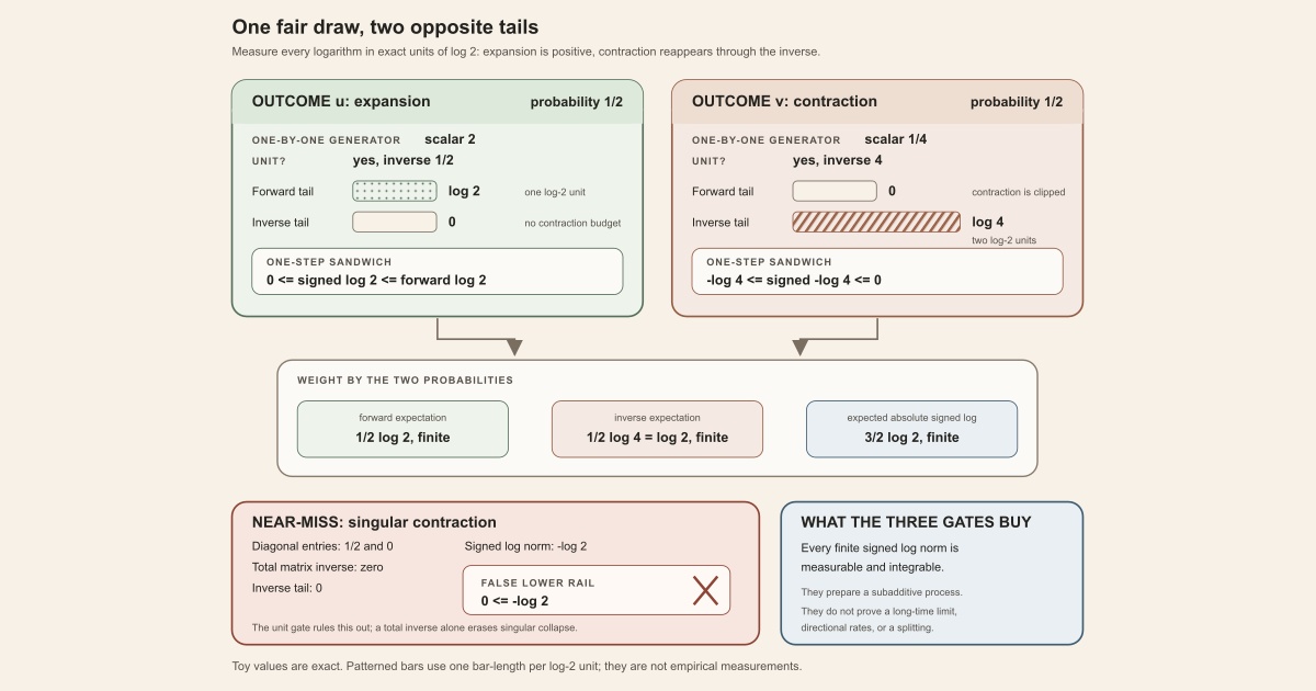
Suppose a fair coin chooses one of two one-by-one matrices:
\[ A(u)=\begin{bmatrix}2\end{bmatrix}, \qquad A(v)=\begin{bmatrix}\tfrac14\end{bmatrix}, \qquad \mathbb P(u)=\mathbb P(v)=\tfrac12. \]The first outcome doubles a vector. The second divides it by four. If we only record expansion, the second outcome looks harmless because its norm is below one. If we also inspect the inverse, its contraction reappears as an expansion by four. Integrable generator log tails are the hypothesis that keeps both of those one-step logarithmic budgets finite.
Work the two outcomes before naming the abstraction
Take the base map to be the identity, so an outcome stays \(u\) or stays \(v\) at every time. The event family is every subset of \(\Omega=\{u,v\}\), and the displayed probabilities define a probability measure : the two masses are nonnegative and add to one. With this discrete event structure, the identity base map and the displayed generator are measurable, and the identity preserves the probability measure. A one-by-one matrix has the absolute value of its entry as its induced infinity operator norm .
For a positive number \(x\), write
\[ \log^+x=\max(0,\log x). \]That is the ordinary paper definition on positive inputs. Lean’s
Real.log is a total function with value zero at zero, so the
formal log⁺ is total too. The singular and empty-dimensional
boundaries below explain why that implementation detail cannot be ignored.
Define three one-step quantities:
\[ F(\omega)=\log^+\lVert A(\omega)\rVert_\infty, \qquad I(\omega)=\log^+\lVert A(\omega)^{-1}\rVert_\infty, \qquad R_1(\omega)=\log\lVert A(\omega)\rVert_\infty. \]Here \(F\) is the forward expansion tail, \(I\) is the inverse contraction tail, and \(R_1\) is the signed logarithmic growth. The complete arithmetic is:
| outcome | probability | generator norm | inverse norm | \(F\) | \(I\) | \(R_1\) |
|---|---|---|---|---|---|---|
| \(u\) | \(1/2\) | \(2\) | \(1/2\) | \(\log 2\) | \(0\) | \(\log 2\) |
| \(v\) | \(1/2\) | \(1/4\) | \(4\) | \(0\) | \(\log 4\) | \(-\log 4\) |
The one-step lower and upper bounds can now be checked without any theorem:
\[ \begin{aligned} u:&\qquad 0\leq \log 2\leq \log 2,\\ v:&\qquad -\log 4\leq-\log 4\leq0. \end{aligned} \]Both tail budgets have finite expectation :
Here expectation is the probability-weighted average of the two values.
\[ \mathbb E[F] =\tfrac12\log2, \qquad \mathbb E[I] =\tfrac12\log4 =\log2. \]The signed logarithm is integrable too, because its expected absolute value is finite:
\[ \mathbb E[|R_1|] =\tfrac12\log2+\tfrac12\log4 =\tfrac32\log2 \lt\infty. \]This last calculation is what ordinary real-valued integrability means on the finite probability space: the function is measurable and the integral of its absolute value is finite. Measurability and integrability are different questions in general. On this finite space with every subset declared an event, every real-valued function is measurable; the explicit sums above then settle finiteness.
One more step shows why the condition propagates
Because the base map is the identity, the horizon-two products are
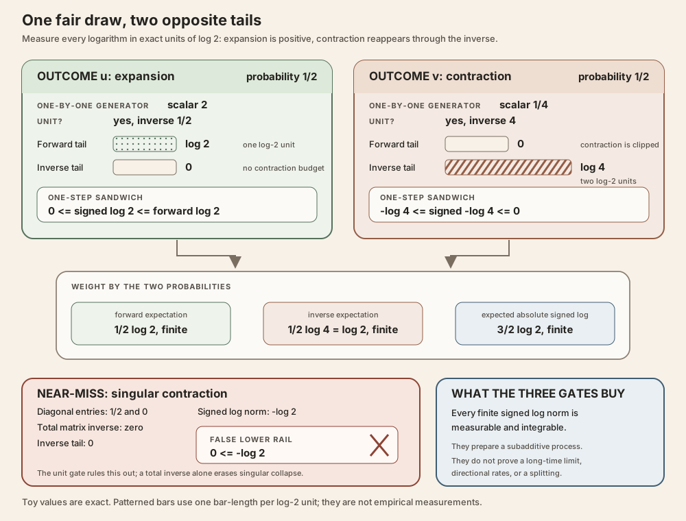
\[ C(2,u)=\begin{bmatrix}4\end{bmatrix}, \qquad C(2,v)=\begin{bmatrix}\tfrac1{16}\end{bmatrix}. \]At \(u\), the two inverse-tail terms are both zero. At \(v\), each is \(\log4\). Therefore the horizon-two sandwich is
\[ \begin{aligned} u:&\qquad 0\leq \log4\leq\log4,\\ v:&\qquad -2\log4=-\log16\leq-\log16\leq0. \end{aligned} \]The example is deliberately small, but the mechanism is already complete: one-step tail budgets become finite sums along the orbit, and the signed log norm sits between them.
Prerequisites in plain language
The general definition combines algebra, probability, and analysis. The following distinctions prevent the notation from doing too much at once.
- A sample space \(\Omega\) is the set of possible base states. An event is a measurable subset of that space.
- A measure \(\mu\) assigns sizes to measurable events. It need not have total mass one. A probability measure does.
- A measurable function respects the selected event structures. Measurability makes the function eligible for integration; it does not say that the function has a finite integral.
- A real-valued function \(f\) is integrable when it is measurable and \(\int |f|\,d\mu\lt\infty\). Positive and negative values cannot hide an infinite tail by cancellation because the absolute value is integrated.
- A square matrix is a unit when it has a multiplicative inverse. For a finite complex square matrix, this is equivalent to nonzero determinant. The project asks for a unit at every base state, not merely outside a null set .
- A measure-preserving transformation \(T:\Omega\to\Omega\) moves the base state without changing the measure. Consequently, composition with \(T^j\) preserves the relevant one-step integrability.
No independence assumption appears in this list. No probability density is required either. The package is formulated for a measure-preserving one-sided discrete matrix cocycle , not specifically for an independent and identically distributed sequence.
The general package
Let \(A(\omega)\) be the one-step generator and let the newest factor appear on the left:
\[ C(k,\omega) =A(T^{k-1}\omega)\cdots A(T\omega)A(\omega), \qquad C(0,\omega)=I. \]For a finite coordinate type \(\iota\), the matrices have complex entries and use the project’s maximum absolute row-sum norm. Define
\[ \begin{aligned} F(\omega)&=\log^+\lVert A(\omega)\rVert_\infty,\\ I(\omega)&=\log^+\lVert A(\omega)^{-1}\rVert_\infty,\\ R_k(\omega)&=\log\lVert C(k,\omega)\rVert_\infty. \end{aligned} \]The integrable-generator-log-tails package has three fields:
| field | paper condition | job |
|---|---|---|
isPointwiseInvertible | \(A(\omega)\) is a unit for every \(\omega\) | makes the inverse lower bound valid |
hasIntegrableGeneratorLogPlus | \(F\in L^1(\mu)\) | controls large one-step expansion |
integrable_inverseGeneratorLogPlus | \(I\in L^1(\mu)\) | controls deep one-step contraction |
The exact proposition-valued structure in the pinned Random Matrix Theory milestone RMT-34 source is:
structure HasIntegrableGeneratorLogTails
    (C : DiscreteMatrixCocycle (ι := ι) μ) : Prop where
  isPointwiseInvertible : C.IsPointwiseInvertible
  hasIntegrableGeneratorLogPlus : C.HasIntegrableGeneratorLogPlus
  integrable_inverseGeneratorLogPlus :
    Integrable C.inverseGeneratorLogPlusNormObservable μ
The structure stores proofs, not extra cocycle data. It does not change the base map, choose inverses, or construct negative-time dynamics.
Why the two analytic fields are separate
The function \(\log^+x\) clips every nonpositive logarithm to zero. A strong contraction can therefore disappear from \(F\). Applying the same operation to the inverse makes that contraction visible in \(I\).
For a nonzero scalar \(a\), measured in a one-by-one matrix,
\[ F=\max(0,\log|a|), \qquad I=\max(0,-\log|a|). \]These are exactly the positive and negative tails of \(\log|a|\). In higher dimension the interpretation is not perfectly symmetric: the forward norm captures the strongest expansion, while the inverse norm captures the strongest contraction. Neither field implies the other.
The finite-time sandwich
For a horizon \(k\in\mathbb N\), define the inverse orbit budget and forward envelope by
\[ S_k^-(\omega) =\sum_{j=0}^{k-1}I(T^j\omega), \qquad P_k(\omega) =\log^+\lVert C(k,\omega)\rVert_\infty. \]The three fields give the pointwise inequality
\[ \boxed{ -S_k^-(\omega) \leq R_k(\omega) \leq P_k(\omega)}. \]The upper rail is the elementary inequality \(\log x\leq\log^+x\). The lower rail uses genuine inverses. For a nonzero finite product,
\[ 1\leq \lVert C(k,\omega)^{-1}\rVert_\infty \lVert C(k,\omega)\rVert_\infty. \]Taking logarithms bounds \(R_k\) from below by the negative inverse-product log norm. Norm submultiplicativity then bounds that inverse-product quantity by the sum \(S_k^-\). The order of the two inequalities reverses when the inverse quantity is negated.
Measure preservation makes every transported one-step tail integrable. Hence \(S_k^-\) is a finite sum of integrable functions, and the forward-tail field makes \(P_k\) integrable. The signed function \(R_k\) is measurable, so an integrable lower rail and upper rail imply
\[ R_k\in L^1(\mu) \qquad\text{for every finite }k. \]No probability normalization or ergodicity is needed for this finite-horizon result.
In Lean: read the conclusion in three languages
hC.integrable_realLogNormObservable khCis a proof ofC.HasIntegrableGeneratorLogTails, so it carries all three fields.- The dot in
hC.integrable_realLogNormObservableselects the theorem whose first explicit proof argument ishC. k : ℕis the finite time horizon.C.realLogNormObservable kis the function \(\omega\mapsto\log\lVert C(k,\omega)\rVert_\infty\).- The theorem’s result is
Integrable (C.realLogNormObservable k) μ. The finalμtells Lean which measure defines integrability.
Here is the complete exact source theorem. The proof first supplies measurability, then the eventual lower and upper inequalities, then the integrability of the two rails:
theorem HasIntegrableGeneratorLogTails.integrable_realLogNormObservable
    {C : DiscreteMatrixCocycle (ι := ι) μ}
    (hC : C.HasIntegrableGeneratorLogTails) (k : ℕ) :
    Integrable (C.realLogNormObservable k) μ := by
  exact MeasureTheory.integrable_of_le_of_le
    (C.measurable_realLogNormObservable k).aestronglyMeasurable
    (Filter.Eventually.of_forall fun ω ↦
      hC.isPointwiseInvertible.neg_inverseOrbitLogPlusSum_le_realLogNormObservable k ω)
    (Filter.Eventually.of_forall fun ω ↦
      C.realLogNormObservable_le_logPlusNormObservable k ω)
    (hC.integrable_inverseOrbitLogPlusSum k).neg
    (hC.hasIntegrableGeneratorLogPlus.integrable_logPlusNormObservable k)
The word Eventually here packages pointwise inequalities in the
almost-everywhere filter interface expected by the integrability theorem. The
proofs were built with of_forall, so these particular inequalities
hold at every \(\omega\), not merely
almost everywhere
.
A tiny standalone Lean worksheet a human can type
Standalone tutorial. The two matrices are powers of two, so the worksheet records each signed logarithm by its exact integer coefficient of \(\log2\). Thus \(2\) has coefficient \(1\), while \(1/4=2^{-2}\) has coefficient \(-2\). This checks the arithmetic and the sandwich without importing Mathlib, Lean’s community mathematics library, defining matrices, or claiming to prove measure-theoretic integrability.
Save the following as GeneratorLogTailsTutorial.lean:
import Std

inductive Outcome where
  | expand
  | contract
deriving Repr, DecidableEq

-- Exact coefficients of log 2: log 2 = 1 unit, log (1/4) = -2 units.
def signedLogUnits : Outcome → Int
  | .expand => 1
  | .contract => -2

def positivePart (z : Int) : Int :=
  if 0 ≤ z then z else 0

def forwardTailUnits (ω : Outcome) : Int :=
  positivePart (signedLogUnits ω)

def inverseTailUnits (ω : Outcome) : Int :=
  positivePart (-signedLogUnits ω)

def sandwichHolds (ω : Outcome) : Bool :=
  decide (-inverseTailUnits ω ≤ signedLogUnits ω ∧
    signedLogUnits ω ≤ forwardTailUnits ω)

def absoluteSignedLogUnits (ω : Outcome) : Nat :=
  (signedLogUnits ω).natAbs

def totalAbsoluteSignedLogUnits : Nat :=
  absoluteSignedLogUnits .expand + absoluteSignedLogUnits .contract

def horizonSignedLogUnits (k : Nat) (ω : Outcome) : Int :=
  (k : Int) * signedLogUnits ω

def horizonInverseBudgetUnits (k : Nat) (ω : Outcome) : Int :=
  (k : Int) * inverseTailUnits ω

def horizonForwardBudgetUnits (k : Nat) (ω : Outcome) : Int :=
  (k : Int) * forwardTailUnits ω

def horizonSandwichHolds (k : Nat) (ω : Outcome) : Bool :=
  decide (-horizonInverseBudgetUnits k ω ≤ horizonSignedLogUnits k ω ∧
    horizonSignedLogUnits k ω ≤ horizonForwardBudgetUnits k ω)

#eval (forwardTailUnits .expand, inverseTailUnits .expand,
  signedLogUnits .expand)
#eval (forwardTailUnits .contract, inverseTailUnits .contract,
  signedLogUnits .contract)
#eval sandwichHolds .expand
#eval sandwichHolds .contract
#eval totalAbsoluteSignedLogUnits
#eval horizonSandwichHolds 2 .expand
#eval horizonSandwichHolds 2 .contract

example : forwardTailUnits .expand = 1 := by decide
example : inverseTailUnits .contract = 2 := by decide
example : totalAbsoluteSignedLogUnits = 3 := by decide
example : horizonSignedLogUnits 2 .contract = -4 := by decide
From the directory containing that file, type:
source "$HOME/.elan/env"
elan run leanprover/lean4:v4.32.0 lean GeneratorLogTailsTutorial.lean
The first two outputs should be (1, 0, 1) and
(0, 2, -2). The next two and the two horizon checks should be
true, and the absolute-log total should be 3. Since
the outcomes are equally likely, dividing that total by two recovers the
paper value \((3/2)\log2\).
This tutorial is safe for an ordinary Mac or Linux machine because it imports
only Std. It does not check the project’s matrices, norms,
measures, logarithms, or integrability theorem.
Try the exact declarations in the project
Full project check. This uses the repository’s pinned Lean and Mathlib dependencies and may require substantial disk space and memory. Create a temporary project worksheet containing:
import NonlinearDynamics.Random.RandomCocycles.RealLogNormIntegrability

#check NonlinearDynamics.Random.RandomCocycles.DiscreteMatrixCocycle.IsPointwiseInvertible
#check NonlinearDynamics.Random.RandomCocycles.DiscreteMatrixCocycle.HasIntegrableGeneratorLogPlus
#check NonlinearDynamics.Random.RandomCocycles.DiscreteMatrixCocycle.HasIntegrableGeneratorLogTails
#check NonlinearDynamics.Random.RandomCocycles.DiscreteMatrixCocycle.measurable_inverseGeneratorLogPlusNormObservable
#check NonlinearDynamics.Random.RandomCocycles.DiscreteMatrixCocycle.IsPointwiseInvertible.neg_inverseOrbitLogPlusSum_le_realLogNormObservable
#check NonlinearDynamics.Random.RandomCocycles.DiscreteMatrixCocycle.realLogNormObservable_le_logPlusNormObservable
#check NonlinearDynamics.Random.RandomCocycles.DiscreteMatrixCocycle.HasIntegrableGeneratorLogTails.integrable_realLogNormObservable
#check NonlinearDynamics.Random.RandomCocycles.DiscreteMatrixCocycle.HasIntegrableGeneratorLogTails.isIntegrableSubadditiveProcessCandidate
#check NonlinearDynamics.Random.RandomCocycles.DiscreteMatrixCocycle.HasIntegrableGeneratorLogPlus.ae_tendsto_normalizedRealLogNormObservable_of_pos
Each #check asks the pinned elaborator for the exact type of a
declaration. The long namespace identifies the declarations without relying on
local open commands. The full-project command below checks the complete
authoritative RMT-34 module with the repository’s pinned Lean and Mathlib
dependencies installed.
cd formalization
lake env lean -DwarningAsError=true NonlinearDynamics/Random/RandomCocycles/RealLogNormIntegrability.lean
Resource note: this exact file uses the repository's
pinned Lean and Mathlib dependencies. Initial project setup can require
substantial disk space and build time. For a lightweight first step on
macOS or Linux, use the page's standalone Lean-core or Std
tutorial.
Why this condition matters for cocycle growth
The signed process is shifted-subadditive when a long interval costs no more than its two consecutive pieces:
\[ R_{m+k}(\omega) \leq R_k(T^m\omega)+R_m(\omega). \]Subadditive growth theory studies the normalized signed quantity
\[ \frac1k\log\lVert C(k,\omega)\rVert_\infty. \]Before an ergodic theorem can control its long-time behavior, the finite-time functions must be analytically usable. The tail package provides exactly two pieces of infrastructure:
integrable_realLogNormObservableproves every finite signed log norm is integrable.isIntegrableSubadditiveProcessCandidatecombines that integrability with shifted subadditivity.
The released RMT-35 vertical slice then adds a probability base and the
project’s pre-ergodic invariant-set condition. Its signed Kingman endpoint is
named
HasIntegrableGeneratorLogTails.ae_tendsto_normalizedRealLogNormObservable.
Under those extra assumptions, it states almost-everywhere convergence to a
deterministic integrated signed growth rate.
That downstream theorem explains why the present hypothesis is valuable, but it must not be read backward into this page. This page’s pinned source and hash cover RMT-34 only. RMT-35 has its own teaching layer; the tail package by itself proves no asymptotic convergence.
Near-misses and boundary cases
Near-miss 1: a singular contraction fools the total inverse
Mathlib’s nonsingular matrix inverse is a total function: on a singular matrix it returns the zero matrix. Take
\[ A= \begin{bmatrix} \tfrac12&0\\ 0&0 \end{bmatrix}. \]Its norm is \(1/2\), so its signed one-step log is \(-\log2\). Its total inverse is zero, whose inverse log-positive tail is \(0\). Without the unit condition, the proposed lower rail would say
\[ 0\leq-\log2, \]which is false. Inverse-tail integrability alone does not rule out singular collapse. Pointwise units make the lower rail meaningful.
Near-miss 2: the forward field does not control contraction
There is a compiled probability-space counterexample in RMT-34. Let \(\Omega=\mathbb N\), give \(n\) probability \(2^{-n-1}\), use the identity base, and choose the one-dimensional generator
\[ A(n)=\begin{bmatrix}\exp(-2^n)\end{bmatrix}. \]Every generator is a unit and every norm is below one, so \(F(n)=0\). The forward tail is integrable. But
\[ I(n)=2^n, \qquad |R_1(n)|=2^n, \qquad 2^{-n-1}2^n=\tfrac12. \]Every outcome contributes the same \(1/2\) to the absolute integral, so the infinite series diverges. The inverse field and signed one-step integrability both fail. This is a probability example, but it is not independent and identically distributed and the identity base is not ergodic. It separates the hypotheses; it does not model repeated independent sampling.
Near-miss 3: almost-everywhere invertibility is not this package
The structure requires ∀ ω, IsUnit (C.generator ω). A statement
that the generator is a unit outside a null set is weaker. One may eventually
develop an almost-everywhere representative interface, but it would need its
own proof that finite products and pointwise lower bounds are valid on a
common full-measure set. It cannot be substituted silently for the current
field.
Boundary 1: inversion reverses matrix order
Because the cocycle puts the newest factor on the left,
\[ C(k,\omega)^{-1} =A(\omega)^{-1}\cdots A(T^{k-1}\omega)^{-1}. \]The scalar log-norm estimate can add the inverse-tail terms in any order, but the matrix product itself cannot. RMT-34 therefore does not claim that these inverse generators form a same-base one-sided inverse cocycle.
Boundary 2: empty matrix dimension is totalized to zero
If the finite coordinate type has no elements, the unique square matrix is both zero and identity. It is a unit, while the selected row-sum norm is zero. Mathlib’s total real logarithm has \(\log0=0\), so every real-log and log-positive observable in this branch is zero. The public theorem handles this type-level case separately, and the sandwich becomes \(0\leq0\leq0\).
Boundary 3: a positive-rate shortcut is a different theorem
RMT-34 also proves that if the earlier log-positive growth rate is strictly positive, then normalized log-positive and signed real logs eventually agree almost everywhere. That route needs neither pointwise inverses nor the inverse tail field. It cannot handle zero clipped rate or negative signed growth, so it does not replace the two-sided tail package.
What this page does not claim
- Integrable one-step tails do not imply independence or identical distribution.
- The three fields alone do not imply ergodicity or a deterministic limit.
- Finite-horizon \(L^1\) membership is not \(L^1\) convergence as \(k\to\infty\).
- The inverse norm does not identify every Lyapunov exponent, an asymptotic exponential growth rate, or construct an Oseledets splitting, a measurable decomposition into directions with different rates.
- Pointwise units do not construct an invertible two-sided base system.
- The small
Stdworksheet checks integer arithmetic only. The full-project command is the check for the exact Mathlib-backed source.
Check your understanding
Why is the forward tail zero at \(A(v)=[1/4]\)?
Because \(\log(1/4)=-\log4\lt0\), and \(\log^+\) replaces negative values by zero.
Why is the inverse tail \(\log4\) at the same outcome?
The inverse is \([4]\), whose norm is \(4\), so its positive logarithm is \(\log4\).
Which field fails in the geometric counterexample?
The inverse-tail integrability field fails. The unit field and the forward log-positive integrability field both hold.
Why is measurability not enough?
A measurable function can still have infinite absolute integral. The geometric inverse tail is measurable but not integrable.
What extra ingredients are needed before reading the RMT-35 asymptotic conclusion?
In addition to the tail package, the theorem uses a probability measure and the project’s pre-ergodic condition for the preserved base.
Where to continue
The log-positive integrability envelope develops the forward field and its finite orbit-sum majorant. The extended log-norm observable explains the zero-faithful extended-real value that the total real logarithm does not retain. The ergodic probability base separates probability normalization from invariant-set rigidity.
Finite-Horizon Log-Positive Cocycle Integrability derives the forward majorant in detail. The Forward-and-Inverse Tail Sandwich for Finite-Time Real Log Norms turns the present mechanism into a longer textbook ascent.
The RMT-34 Development Notebook records source-order engineering decisions and proof boundaries.
References
Nonlinear Dynamics Lean project.
Site-hosted RMT-34 checked source,
with repository provenance at
commit 624c727146532d3b2656f5f23136557d5779b4fd,
RealLogNormIntegrability.lean. This is the authoritative source
for the three-field structure, finite-time sandwich, singular and empty
boundaries, geometric counterexample, and positive-rate shortcut described on
this page.
Mathlib contributors.
Geometric probability measures,
Mathlib 4. This pinned source defines geometricMeasure, proves its
probability-measure instance, computes singleton masses, and supplies the
weighted-series integrability test used by the compiled counterexample.
Mathlib contributors.
Total nonsingular matrix inverse,
Mathlib 4. This pinned source defines the determinant-adjugate total inverse,
proves its zero value on singular matrices, characterizes matrix units, and
proves the product-order theorem Matrix.mul_inv_rev.
Mathlib contributors.
Positive logarithm,
Mathlib 4. This pinned source defines Real.posLog as the maximum of
zero and the total real logarithm and proves the product bound used for finite
orbit majorants.
Mathlib contributors.
Bochner integrability bounds,
Mathlib 4. The theorem integrable_of_le_of_le turns measurable
control by an integrable lower and upper function into integrability of the
sandwiched real-valued function.
J. F. C. Kingman. The Ergodic Theory of Subadditive Stochastic Processes, Journal of the Royal Statistical Society, Series B 30(3), 1968, 499-510. This is the classical asymptotic destination for integrable subadditive processes. The RMT-34 package prepares an input interface rather than reproving the classical theorem.
V. I. Oseledets. A Multiplicative Ergodic Theorem: Characteristic Lyapunov Exponents of Dynamical Systems, Transactions of the Moscow Mathematical Society 19, 1968, 197-231. This is the classical source for measurable Lyapunov splittings. RMT-34 proves neither a spectrum nor a splitting.
The exact upstream Lean revision audited for this page is Mathlib commit
81a5d257,
the revision pinned by formalization/lake-manifest.json.