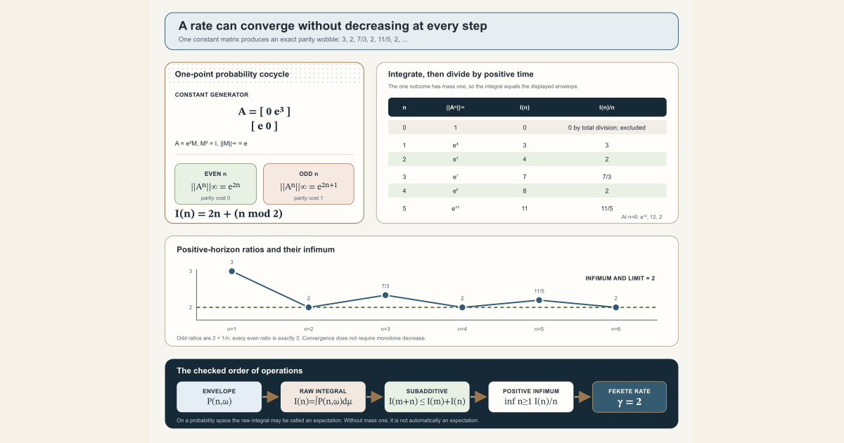
First compute a growth rate that wobbles
Take the one-point sample space
\[ \Omega=\{\star\}, \qquad \mu(\{\star\})=1, \]and let the base transformation fix its only point: \(T(\star)=\star\). Because the whole space has mass one, \(\mu\) is a probability measure .
Use the same \(2\times2\) matrix at every step. This is a constant one-sided matrix cocycle :
\[ A= \begin{bmatrix} 0&e^3\\ e&0 \end{bmatrix} {} = e^2 \begin{bmatrix} 0&e\\ e^{-1}&0 \end{bmatrix} =e^2M. \]Here \(e\) is the base of the natural logarithm. These real entries can be viewed as complex entries, as in the project’s cocycle type. The norm is the maximum absolute row-sum norm . Direct multiplication and those row sums give
\[ M^2=I, \qquad \lVert M\rVert_\infty=e, \qquad A^2=e^4I. \]Even powers lose the extra \(M\); odd powers retain it:
\[ \lVert A^n\rVert_\infty {} = \begin{cases} e^{2n},&n\text{ even},\\ e^{2n+1},&n\text{ odd}. \end{cases} \]The finite-horizon log-positive envelope is
\[ P_n(\star)=\log^+\lVert A^n\rVert_\infty. \]Here \(\log^+x=\max\{0,\log x\}\): it retains expansion above one and clips nonpositive logarithms to zero. Every displayed norm is at least one, so the positive part does not clip its logarithm. The one point has mass one, so integrating does not change the number. If
\[ I_n=\int_\Omega P_n(\omega)\,d\mu(\omega), \]then
\[ \boxed{I_n=2n+(n\bmod 2)}. \]Here \(n\bmod2\) is the remainder after division by two: zero for even \(n\) and one for odd \(n\).
| Horizon \(n\) | \(\lVert A^n\rVert_\infty\) | Integrated value \(I_n\) | Lean’s totalized \(I_n/n\) | Included in the rate infimum? |
|---|---|---|---|---|
| \(0\) | \(1\) | \(0\) | \(0/0=0\) | no |
| \(1\) | \(e^3\) | \(3\) | \(3\) | yes |
| \(2\) | \(e^4\) | \(4\) | \(2\) | yes |
| \(3\) | \(e^7\) | \(7\) | \(7/3\) | yes |
| \(4\) | \(e^8\) | \(8\) | \(2\) | yes |
| \(5\) | \(e^{11}\) | \(11\) | \(11/5\) | yes |
| \(6\) | \(e^{12}\) | \(12\) | \(2\) | yes |
The normalized sequence is not decreasing:
\[ 3,\ 2,\ \frac73,\ 2,\ \frac{11}{5},\ 2,\ldots \]Every even positive horizon has ratio \(2\). Every odd horizon has ratio \(2+1/n\). Therefore
\[ \inf_{n\ge1}\frac{I_n}{n}=2 \qquad\text{and}\qquad \lim_{n\to\infty}\frac{I_n}{n}=2. \]This value \(2\) is the integrated log-positive growth rate of the example.
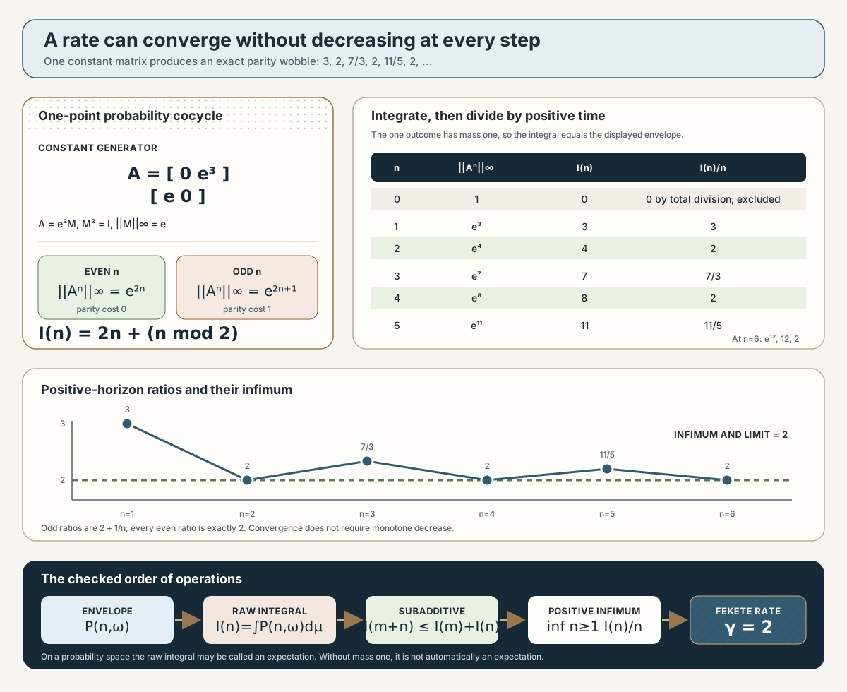
Check subadditivity by parity
A real sequence \(u:\mathbb N\to\mathbb R\) is subadditive when
\[ u_{m+n}\leq u_m+u_n \qquad\text{for every }m,n\in\mathbb N. \]For the example, write \(r_n=n\bmod2\). The remainder obeys
\[ r_{m+n}\leq r_m+r_n. \]This can be checked in four parity cases. If \(m\) and \(n\) are both odd, the left remainder is zero while the right remainders sum to two. In the other three cases the two sides are equal. Consequently,
\[ \begin{aligned} I_{m+n} &=2(m+n)+r_{m+n}\\ &\leq2m+2n+r_m+r_n\\ &=I_m+I_n. \end{aligned} \]Subadditivity says that treating a combined block at once costs no more than adding the separate block budgets. It does not say \(I_{m+n}=I_m+I_n\), and it does not force \(I_n/n\) to decrease at every step.
General definition
An integrated log-positive growth rate is a deterministic asymptotic rate built from a matrix cocycle by integrating before taking a limit. For a cocycle \(C\), horizon \(k\), and base state \(\omega\), define the finite-horizon positive-log envelope
\[ P_k(\omega) {} = \log^+\lVert C(k,\omega)\rVert_\infty. \]The project’s IntegratedLogPlusGrowth.lean module, called RMT-16
in the historical checkpoint ledger, defines the scalar sequence
and, under the explicit one-step
integrability
hypothesis from the preceding
LogPlusIntegrability.lean module, called RMT-15 in that ledger,
proves
Mathlib’s deterministic Fekete theorem then supplies
\[ \gamma_\mu^+(C) {} = \lim_{k\to\infty}\frac{I_k}{k} {} = \inf_{k\ge 1}\frac{I_k}{k}. \]The notation \(\gamma_\mu^+(C)\) is explanatory prose. Lean calls the value
integratedLogPlusGrowthRate C hC, where hC records
one-step positive-log integrability. Its exact proposition is
Integrable (C.logPlusNormObservable 1) μ
It says the one-step envelope is strongly measurable almost everywhere and has finite integral of its absolute value. Because the envelope is nonnegative, this is precisely the finite positive-tail condition needed by the finite-horizon propagation argument.
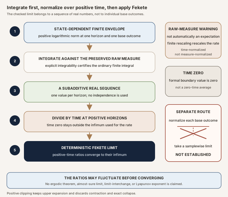
Three objects that must not be merged
| Object | Lean expression | Type | Dependence |
|---|---|---|---|
| Finite envelope \(P_k(\omega)\) | C.logPlusNormObservable k ω | \(\mathbb R\) | Horizon and base point |
| Integrated value \(I_k\) | C.integratedLogPlusNorm k | \(\mathbb R\) | Horizon only |
| Normalized value \(A_k\) | C.normalizedIntegratedLogPlusNorm k | \(\mathbb R\) | Horizon only |
The theorem follows the top-to-bottom direction in this table. It first removes \(\omega\) by integration, then studies the numerical sequence \(I_k/k\). It does not fix \(\omega\) and study \(P_k(\omega)/k\).
The totalized-integral warning
Mathlib’s real-valued Bochner integral is a total function. If its integrand
is not integrable, the integral is defined to be zero. This convention is
recorded by MeasureTheory.integral_undef.
Consequently, integratedLogPlusNorm can be defined for every
cocycle and every horizon without an integrability premise. Its codomain
\(\mathbb R\) does not by itself certify a finite analytic moment. Likewise,
the unconditional theorem \(0\le I_k\) can reduce to the harmless fact
\(0\le0\) in a nonintegrable case.
For example, on an infinite-measure space the constant function one need not be integrable. Mathlib still assigns its totalized Bochner integral the real value zero. Calling that value a finite growth moment would hide the failed hypothesis.
How the shift disappears
RMT-15 supplies the pointwise cocycle estimate
\[ P_{m+k}(\omega) \le P_k(T^m\omega)+P_m(\omega). \]The later block really begins at \(T^m\omega\), so the shift cannot be erased pointwise. Every natural iterate of \(T\) preserves \(\mu\), however. Ordinary measurability, the mapped-measure equality, and Mathlib’s totalized integral make the pullback identity unconditional:
\[ \int_\Omega P_k(T^m\omega)\,d\mu(\omega) {} = \int_\Omega P_k(\omega)\,d\mu(\omega) {} = I_k. \]Without integrability, both sides of this identity may only be totalized zeros.
Under hC, the finite envelopes are integrable, so integrating the
pointwise estimate legitimately gives \(I_{m+k}\le I_m+I_k\). Preservation has
identified shifted integrals. It has not created integrability, probability,
independence, identical distribution, or ergodicity.
The finite orbit-sum majorant from RMT-15 also integrates exactly:
\[ S_k(\omega) {} = \sum_{j=0}^{k-1}P_1(T^j\omega), \qquad \int_\Omega S_k\,d\mu=kI_1. \]Since \(P_k\le S_k\), RMT-16 obtains \(I_k\le kI_1\). Neither equality nor inequality needs independent orbit terms.
Fekete’s lemma in plain language
An infimum is the greatest lower bound. For example, the positive-horizon ratios in the opening calculation all lie at or above \(2\), and no larger number is below all of them because the even ratios equal \(2\). Their infimum is therefore \(2\).
Mathlib’s real-valued form of Fekete’s lemma starts with a sequence \(u:\mathbb N\to\mathbb R\) satisfying
\[ u_{m+n}\leq u_m+u_n. \]It also asks that the normalized range
\[ \left\{\frac{u_n}{n}:n\in\mathbb N\right\} \]be bounded below. It then proves
\[ \lim_{n\to\infty}\frac{u_n}{n} {} = \inf_{n\geq1}\frac{u_n}{n}. \]The project discharges the lower-bound condition with zero because every log-positive envelope and every integrated value is nonnegative. Its sequence is \(u_n=I_n\).
Fekete’s lemma is deterministic. Once the integrals \(I_n\) have been formed, the theorem is applied only to that real sequence. Its statement contains no sample space, base transformation, matrix, or individual outcome.
Time zero is a boundary convention
Lean defines
\[ A_k=\frac{I_k}{(k:\mathbb R)} \]for every natural \(k\). At time zero, \(I_0=0\) and real division is total, so \(A_0=0/0=0\). This is a formal boundary value, not growth per zero units of time.
Mathlib avoids that interpretation in its definition of the Fekete rate:
sInf ((fun n : ℕ => u n / n) '' Set.Ici 1)
Thus the infimum ranges over \(k\ge1\). It is not the infimum of the entire range of \(A\). That difference can change the answer: because \(A_0=0\) and every \(A_k\ge0\), the infimum of the full range would always be zero, even when every positive-time ratio equals a positive constant.
Fekete convergence also does not say that the ratios decrease monotonically. The opening sequence visibly fluctuates. Nor must the infimum be a minimum attained at one horizon; the opening example happens to attain it at every positive even horizon, but that is extra structure.
Raw measure is not expectation
The cocycle is parameterized by a raw measure \(\mu\). Its structure contains no probability assumption, no finite-mass hypothesis, and no division by \(\mu(\Omega)\). Therefore \(I_k\) is a raw integral, not automatically an expectation , and \(I_k/k\) is normalized in time only.
Finite scalar rescaling makes the distinction visible. If a finite nonnegative scalar \(c\) is used to repackage the same cocycle over \(c\mu\), then Mathlib’s measure-scaling and integral-scaling APIs imply that the integrated values, normalized values, and resulting rate scale by \(c\), provided the corresponding integrability conditions are handled. For \(c\gt0\), integrability is equivalent before and after rescaling. For \(c=0\), every integral vanishes and the rescaled measure makes every function integrable. Scaling by an infinite extended scalar is outside this statement.
This finite-rescaling observation is an upstream consequence, not one of the thirteen exported RMT-16 declarations. Avoid the broader phrase “scales with total measure,” especially when \(\mu(\Omega)=\infty\).
Expectation language becomes justified only after separately establishing
that \(\mu\) is a probability measure, meaning \(\mu(\Omega)=1\). The
successor module introduces
finiteHorizonLogPlusExpectation under exactly that typeclass and
proves it is the same scalar as integratedLogPlusNorm. Even then,
the current theorem gives a limit of finite-horizon expectations, not an
expectation of a proved samplewise limit.
Edge cases that change the reading
Take a one-point base whose raw measure has finite, strictly positive mass \(q\), and take a constant one-dimensional generator \(\lambda\gt1\). Then
\[ P_k=k\log\lambda, \qquad I_k=qk\log\lambda, \qquad A_k=q\log\lambda \quad(k\ge1). \]Hence
\[ \gamma_\mu^+(C)=q\log\lambda. \]Doubling \(q\) doubles the integrated rate without changing the dynamics. The example also isolates the time-zero trap: \(A_0=0\), but the positive-time infimum is \(q\log\lambda\), which is strictly positive.
If instead \(0\lt\lambda\lt1\), every positive-log envelope is zero and the RMT-16 rate is zero, while the ordinary logarithmic growth rate \(\log\lambda\) is negative. Positive clipping has erased contraction.
A sharper collapse example uses the constant matrix
\[ B= \begin{bmatrix} 0&2\\ 0&0 \end{bmatrix}. \]Its selected row-sum norm is two, but \(B^2=0\). The one-step envelope is \(\log2\), every envelope from time two onward is zero, and the integrated log-positive growth rate is zero. One-step expansion and later exact collapse are both compatible with a zero RMT-16 rate.
These are algebraic teaching examples, not empirical random-matrix data.
The thirteen-declaration interface
RMT-16 exports the following declarations in source order:
| No. | Declaration | Exact role |
|---|---|---|
| 1 | integratedLogPlusNorm | Defines the totalized scalar integral \(I_k\) without an integrability premise |
| 2 | integratedLogPlusNorm_zero | Proves \(I_0=0\) unconditionally |
| 3 | integratedLogPlusNorm_nonneg | Proves \(0\le I_k\) unconditionally, without proving integrability |
| 4 | integral_logPlusNormObservable_at_base_iterate_eq | Removes any natural base iterate inside the totalized integral unconditionally; the identity may be \(0=0\) without integrability |
| 5 | HasIntegrableGeneratorLogPlus.integral_orbitLogPlusSum_eq | Proves \(\int S_k\,d\mu=kI_1\) |
| 6 | HasIntegrableGeneratorLogPlus.integratedLogPlusNorm_le_nat_mul | Proves \(I_k\le kI_1\) |
| 7 | HasIntegrableGeneratorLogPlus.integratedLogPlusNorm_add_le | Proves \(I_{m+k}\le I_m+I_k\) |
| 8 | HasIntegrableGeneratorLogPlus.subadditive_integratedLogPlusNorm | Packages \(I\) as a Mathlib Subadditive sequence |
| 9 | normalizedIntegratedLogPlusNorm | Defines \(A_k=I_k/k\) for every natural \(k\) |
| 10 | normalizedIntegratedLogPlusNorm_nonneg | Proves \(0\le A_k\) unconditionally |
| 11 | bddBelow_normalizedIntegratedLogPlusNorm | Uses zero as a lower bound for the full normalized range |
| 12 | integratedLogPlusGrowthRate | Defines the positive-index Fekete infimum under hC |
| 13 | HasIntegrableGeneratorLogPlus.tendsto_normalizedIntegratedLogPlusNorm | Proves deterministic scalar convergence \(A_k\to\gamma_\mu^+(C)\) |
Declarations 1, 2, 3, 4, 9, 10, and 11 are unconditional. Their total
definitions, order properties, and preserved-pullback equality must not be
mistaken for an integrability result. The finite orbit-sum identity, bounds,
subadditivity, rate definition, and convergence all use
HasIntegrableGeneratorLogPlus.
In Lean: from envelope to deterministic rate
1. Form one real number
C.integratedLogPlusNorm kThe exact project definition is:
def integratedLogPlusNorm
    (C : DiscreteMatrixCocycle (ι := ι) μ) (k : ℕ) : ℝ :=
  ∫ ω, C.logPlusNormObservable k ω ∂μ
A human with C and k in scope types:
#check C.integratedLogPlusNorm k
Read the definition token by token:
C.logPlusNormObservable k ωis \(P_k(\omega)\), the nonnegative finite-horizon envelope at outcome \(\omega\);∫ ω, … ∂μis Lean notation for integration with respect to \(\mu\);k : ℕmakes the horizon a natural number;: ℝsays the result is one real scalar; and- no
Integrableargument occurs in the definition, because the Bochner integral is totalized.
2. Turn the cocycle split into scalar subadditivity
hC.integratedLogPlusNorm_add_le m kThe human types:
#check hC.integratedLogPlusNorm_add_le m k
#check hC.subadditive_integratedLogPlusNorm
hChas typeC.HasIntegrableGeneratorLogPlus; it is the explicit analytic certificate that makes integral monotonicity legitimate.integratedLogPlusNorm_add_lereturns the displayed inequality.subadditive_integratedLogPlusNormpackages all choices ofmandkintoSubadditive C.integratedLogPlusNorm.- Method notation puts the proof object
hCbefore the theorem name; it does not change the mathematical statement.
3. Normalize and name the rate
C.normalizedIntegratedLogPlusNorm k; C.integratedLogPlusGrowthRate hCThe two exact definitions are:
def normalizedIntegratedLogPlusNorm
    (C : DiscreteMatrixCocycle (ι := ι) μ) (k : ℕ) : ℝ :=
  C.integratedLogPlusNorm k / k

def integratedLogPlusGrowthRate
    (C : DiscreteMatrixCocycle (ι := ι) μ)
    (hC : C.HasIntegrableGeneratorLogPlus) : ℝ :=
  hC.subadditive_integratedLogPlusNorm.lim
A human types:
#check C.normalizedIntegratedLogPlusNorm k
#check C.integratedLogPlusGrowthRate hC
The natural number k is coerced to a real number by the division
operation. At k = 0, real division returns zero. The protected
Mathlib definition Subadditive.lim uses
Set.Ici 1, the natural numbers at least one, so the rate itself
does not use that artificial time-zero ratio.
4. State convergence and expose the infimum
hC.tendsto_normalizedIntegratedLogPlusNormThe exact proof term has type
Tendsto C.normalizedIntegratedLogPlusNorm atTop
  (𝓝 (C.integratedLogPlusGrowthRate hC))
and a human asks Lean for it with:
#check hC.tendsto_normalizedIntegratedLogPlusNorm
Tendsto f atTop (𝓝 a)says \(f(k)\) tends to \(a\) as natural \(k\) tends to infinity.atTopis the filter describing arbitrarily large horizons.𝓝 ais the neighborhood filter around the proposed real limit.- The theorem has no outcome
ω; it is convergence of a deterministic scalar sequence.
The next project module exposes the rate’s defining infimum:
hC.integratedLogPlusGrowthRate_eq_sInfThe exact conclusion is:
C.integratedLogPlusGrowthRate hC =
  sInf (C.normalizedIntegratedLogPlusNorm '' Set.Ici 1)
Here sInf is the infimum, ’’ is the image of a set
under a function, and Set.Ici 1 is
\(\{k\in\mathbb N:1\leq k\}\). The related theorem
hC.integratedLogPlusGrowthRate_le_normalized hk says the rate is
below every ratio whose horizon proof hk : k ≠ 0 is supplied.
Exact source excerpts
Full project check. This uses the repository’s pinned Lean and Mathlib
dependencies and may require substantial disk space and memory.
The current module defines the
rate through Mathlib’s subadditive limit and proves convergence in
IntegratedLogPlusGrowth.lean:
def integratedLogPlusGrowthRate
    (C : DiscreteMatrixCocycle (ι := ι) μ)
    (hC : C.HasIntegrableGeneratorLogPlus) : ℝ :=
  hC.subadditive_integratedLogPlusNorm.lim

theorem HasIntegrableGeneratorLogPlus.tendsto_normalizedIntegratedLogPlusNorm
    {C : DiscreteMatrixCocycle (ι := ι) μ}
    (hC : C.HasIntegrableGeneratorLogPlus) :
    Tendsto C.normalizedIntegratedLogPlusNorm atTop
      (𝓝 (C.integratedLogPlusGrowthRate hC)) := by
  exact hC.subadditive_integratedLogPlusNorm.tendsto_lim
    C.bddBelow_normalizedIntegratedLogPlusNorm
Resource label: pinned Mathlib. The repository’s pinned
Mathlib/Analysis/Subadditive.lean
contains:
open Set Filter Topology

def Subadditive (u : ℕ → ℝ) : Prop :=
  ∀ m n, u (m + n) ≤ u m + u n

namespace Subadditive

variable {u : ℕ → ℝ} (h : Subadditive u)

protected def lim (_h : Subadditive u) :=
  sInf ((fun n : ℕ => u n / n) '' Ici 1)

theorem tendsto_lim (hbdd : BddBelow (range fun n => u n / n)) :
    Tendsto (fun n => u n / n) atTop (𝓝 h.lim) := by
  refine tendsto_order.2 ⟨fun l hl => ?_, fun L hL => ?_⟩
  · refine eventually_atTop.2
      ⟨1, fun n hn => hl.trans_le (h.lim_le_div hbdd (zero_lt_one.trans_le hn).ne')⟩
  · obtain ⟨n, npos, hn⟩ : ∃ n : ℕ, 0 < n ∧ u n / n < L := by
      rw [Subadditive.lim] at hL
      rcases exists_lt_of_csInf_lt (by simp) hL with ⟨x, hx, xL⟩
      rcases (mem_image _ _ _).1 hx with ⟨n, hn, rfl⟩
      exact ⟨n, zero_lt_one.trans_le hn, xL⟩
    exact h.eventually_div_lt_of_div_lt npos.ne' hn

end Subadditive
The proof first uses the infimum to obtain the eventual lower bound. For an upper neighborhood, it chooses one positive horizon whose ratio is already below that neighborhood and applies the finite block-and-remainder estimate.
Full project check. This uses the repository’s pinned Lean and Mathlib
dependencies and may require substantial disk space and memory.
The successor
ProbabilityErgodicBase.lean
unfolds the positive-horizon infimum:
theorem HasIntegrableGeneratorLogPlus.integratedLogPlusGrowthRate_eq_sInf
    {C : DiscreteMatrixCocycle (ι := ι) μ}
    (hC : C.HasIntegrableGeneratorLogPlus) :
    C.integratedLogPlusGrowthRate hC =
      sInf (C.normalizedIntegratedLogPlusNorm '' Ici 1) := by
  rw [integratedLogPlusGrowthRate, Subadditive.lim]
  rfl
Standalone tutorial: parity worksheet
Standalone tutorial. The following worksheet imports only
Std. It computes the opening sequence exactly, reduces each
positive ratio to a numerator-denominator pair, and checks subadditivity on the
finite square \(0\leq m,n\leq20\). It does not define matrix norms, Bochner
integrals, or prove the infinite Fekete theorem.
Save it as ParityFeketeScratch.lean:
import Std

def integratedValue (n : Nat) : Nat :=
  2 * n + n % 2

structure Fraction where
  numerator : Nat
  denominator : Nat
deriving Repr, BEq

def reduceFraction (a b : Nat) : Fraction :=
  let g := Nat.gcd a b
  { numerator := a / g, denominator := b / g }

def normalized (n : Nat) : Option Fraction :=
  if n = 0 then
    none
  else
    some (reduceFraction (integratedValue n) n)

def subadditiveOn (bound : Nat) : Bool :=
  (List.range (bound + 1)).all fun m =>
    (List.range (bound + 1)).all fun n =>
      decide (integratedValue (m + n) ≤
        integratedValue m + integratedValue n)

def boundedBelowByTwoOn (bound : Nat) : Bool :=
  (List.range (bound + 1)).all fun n =>
    if n = 0 then
      true
    else
      decide (2 * n ≤ integratedValue n)

def horizons : List Nat := [0, 1, 2, 3, 4, 5, 6]

#eval horizons.map fun n => (n, integratedValue n, normalized n)
#eval subadditiveOn 20
#eval boundedBelowByTwoOn 20
Run it on a normal macOS or Linux machine with the pinned small toolchain:
source "$HOME/.elan/env"
elan run leanprover/lean4:v4.32.0 lean ParityFeketeScratch.lean
The ledger reports integrated values \(0,3,4,7,8,11,12\). The time-zero
ratio is none; the positive fractions are
\(3/1,2/1,7/3,2/1,11/5,2/1\). Both finite checks print true.
The parity proof earlier on this page establishes subadditivity for all natural
indices. This finite worksheet is an executable arithmetic audit, not a
replacement for that proof or for Mathlib’s analytic theorem. The exact file
was executed successfully with Lean 4.32.0 while repairing this page: it
printed the displayed seven-row ledger followed by true and
true.
Try it in the repository
Full project check. This uses the repository’s pinned Lean and Mathlib dependencies and may require substantial disk space and memory. Create a temporary project worksheet containing:
import NonlinearDynamics.Random.RandomCocycles.ProbabilityErgodicBase

open MeasureTheory Set Filter Topology
open NonlinearDynamics.Random.RandomCocycles
open scoped Matrix.Norms.Operator Real

universe uΩ uι

variable {Ω : Type uΩ} {ι : Type uι} [MeasurableSpace Ω]
  [Fintype ι] [DecidableEq ι] {μ : Measure Ω}
variable (C : DiscreteMatrixCocycle (ι := ι) μ)
variable (hC : C.HasIntegrableGeneratorLogPlus)
variable (m k : ℕ)

#check MeasureTheory.integral_undef
#check Subadditive
#check Subadditive.lim
#check Subadditive.lim_le_div
#check Subadditive.tendsto_lim
#check C.integratedLogPlusNorm k
#check C.integratedLogPlusNorm_zero
#check C.integratedLogPlusNorm_nonneg k
#check C.integral_logPlusNormObservable_at_base_iterate_eq k m
#check hC.integral_orbitLogPlusSum_eq k
#check hC.integratedLogPlusNorm_le_nat_mul k
#check hC.integratedLogPlusNorm_add_le m k
#check hC.subadditive_integratedLogPlusNorm
#check C.normalizedIntegratedLogPlusNorm k
#check C.normalizedIntegratedLogPlusNorm_nonneg k
#check C.bddBelow_normalizedIntegratedLogPlusNorm
#check C.integratedLogPlusGrowthRate hC
#check hC.tendsto_normalizedIntegratedLogPlusNorm
#check hC.integratedLogPlusGrowthRate_nonneg
#check hC.integratedLogPlusGrowthRate_eq_sInf
#check hC.integratedLogPlusGrowthRate_le_normalized
#check hC.integratedLogPlusGrowthRate_le_oneStep

section Probability

variable [IsProbabilityMeasure μ]

#check C.finiteHorizonLogPlusExpectation hC k
#check hC.finiteHorizonLogPlusExpectation_eq_integratedLogPlusNorm k

end Probability
Each #check asks the pinned elaborator for an exact type. The
current leaf owns the definition and convergence theorem:
cd formalization
lake env lean NonlinearDynamics/Random/RandomCocycles/IntegratedLogPlusGrowth.lean
The successor leaf owns the explicit infimum, upper-bound, and probability-expectation declarations:
cd formalization
lake env lean NonlinearDynamics/Random/RandomCocycles/ProbabilityErgodicBase.lean
Both full project checks use the repository’s pinned Lean and Mathlib dependencies and may require substantial disk space and memory.
cd formalization
lake env lean -DwarningAsError=true NonlinearDynamics/Random/RandomCocycles/IntegratedLogPlusGrowth.lean
Resource note: this exact file uses the repository's
pinned Lean and Mathlib dependencies. Initial project setup can require
substantial disk space and build time. For a lightweight first step on
macOS or Linux, use the page's standalone Lean-core or Std
tutorial.
What this rate does not establish
RMT-16 proves none of the following:
- convergence of \(P_k(\omega)/k\) for any fixed \(\omega\);
- almost-everywhere, in-probability, distributional, or \(L^1\) convergence;
- interchange of a limit and the integral;
- probability normalization, stationarity in a probabilistic sense, or an expected samplewise limit;
- ergodicity, mixing, independence, or identical distribution;
- Kingman’s subadditive ergodic theorem;
- the Furstenberg-Kesten theorem;
- a Lyapunov exponent, spectrum, filtration, or Oseledets splitting;
- contraction, inverse-norm, smallest-singular-value, or negative-log control;
- integrability or convergence for the zero-faithful extended log norm; or
- a derivative cocycle, random Jacobian, or two-sided dynamics.
The checked conclusion is narrower and exact: the sequence of integrated positive-growth envelopes, normalized by time, converges as a deterministic sequence of real numbers.
Exercises
- Multiply the opening matrix by itself and verify every entry of \(A^2=e^4I\).
- Compute \(\lVert A^7\rVert_\infty\), \(I_7\), and \(I_7/7\). Repeat at horizon eight.
- In which parity case is \(I_{m+n}\leq I_m+I_n\) strict? By how much?
- Explain why the time-zero normalized value is defined in Lean but excluded from the rate infimum.
- Replace the one-point probability measure by a one-point raw measure of mass three. What happens to \(I_n\), \(I_n/n\), and the rate?
- The sequence \(u_n=2n+1\) is subadditive. Show that its positive-time ratios converge to an infimum of two that is never attained.
- Explain why “limit of finite-horizon expectations” does not by itself mean “expectation of a samplewise limit.”
- Match each paper object \(P_k(\omega)\), \(I_k\), \(I_k/k\), and \(\gamma_\mu^+(C)\) with its exact Lean identifier.
Where to continue
RMT-34’s Forward-and-Inverse Tail Sandwich adds a precisely guarded real-log endpoint. When this deterministic log-positive rate is strictly positive, RMT-33 convergence forces the finite-time unclipped logarithm to become positive eventually, so the normalized real log converges almost everywhere to the same rate. The theorem does not require matrix invertibility or an inverse-tail moment. It says nothing about a zero or negative signed rate, and its empty-dimensional specialization is vacuous because the present rate is then zero.
The ergodic probability base entry separates the unit-mass, invariant-rigidity, and finite-time integrability roles that the present raw-measure rate intentionally leaves apart.
Probability Normalization and Ergodic Rigidity Before Kingman develops that next interface and explains why it still does not construct a samplewise limit.
Integrated Log-Positive Cocycle Growth and Its Deterministic Fekete Limit derives all thirteen declarations, explains the two proof strands entering Fekete’s theorem, and audits every assumption and nonclaim.
The Guarded Real-Liminf Bridge to Log-Positive Kingman Convergence shows how a later milestone proves that the samplewise normalized log-positive observable converges almost everywhere to this already-defined deterministic rate. That theorem adds substantial ergodic and lower-deviation hypotheses; it does not turn any RMT-16 declaration into a samplewise or signed-growth claim.
Finite-Horizon Log-Positive Cocycle Integrability develops the RMT-15 predecessor. The log-positive integrability envelope entry explains the positive-log clipping and finite orbit majorant on which the present rate depends.
References
Mathlib contributors.
Subadditive and superadditive sequences,
Mathlib 4 documentation. This official source defines
Subadditive.lim by a positive-index infimum and proves convergence
of the normalized sequence under a lower-bound hypothesis.
Mathlib contributors. The Bochner integral, Mathlib 4 documentation. This official source records totalization for nonintegrable functions and supplies integral monotonicity, finite linearity, pullback, and finite measure-scaling results used by this layer.
Mathlib contributors. Measure-preserving maps, Mathlib 4 documentation. This official source gives pushforward equality, natural-iterate preservation, and preservation after finite scalar measure rescaling.
M. Fekete. Über die Verteilung der Wurzeln bei gewissen algebraischen Gleichungen mit ganzzahligen Koeffizienten, Mathematische Zeitschrift 17, 228-249, 1923. This is the historical primary source associated with the deterministic subadditive lemma.
J. F. C. Kingman. The ergodic theory of subadditive stochastic processes, Journal of the Royal Statistical Society: Series B 30(3), 499-510, 1968. This primary source establishes a later stochastic theorem under additional hypotheses. RMT-16 does not invoke it.
Harry Furstenberg and Harry Kesten. Products of Random Matrices, The Annals of Mathematical Statistics 31(2), 457-469, 1960. This primary source motivates asymptotic random-matrix-product growth; none of its samplewise conclusions is proved here.
The exact upstream Lean source audited for this entry is Mathlib commit
81a5d257,
the revision pinned by formalization/lake-manifest.json.