Start with six states and two sealed cycles
Let the state space be
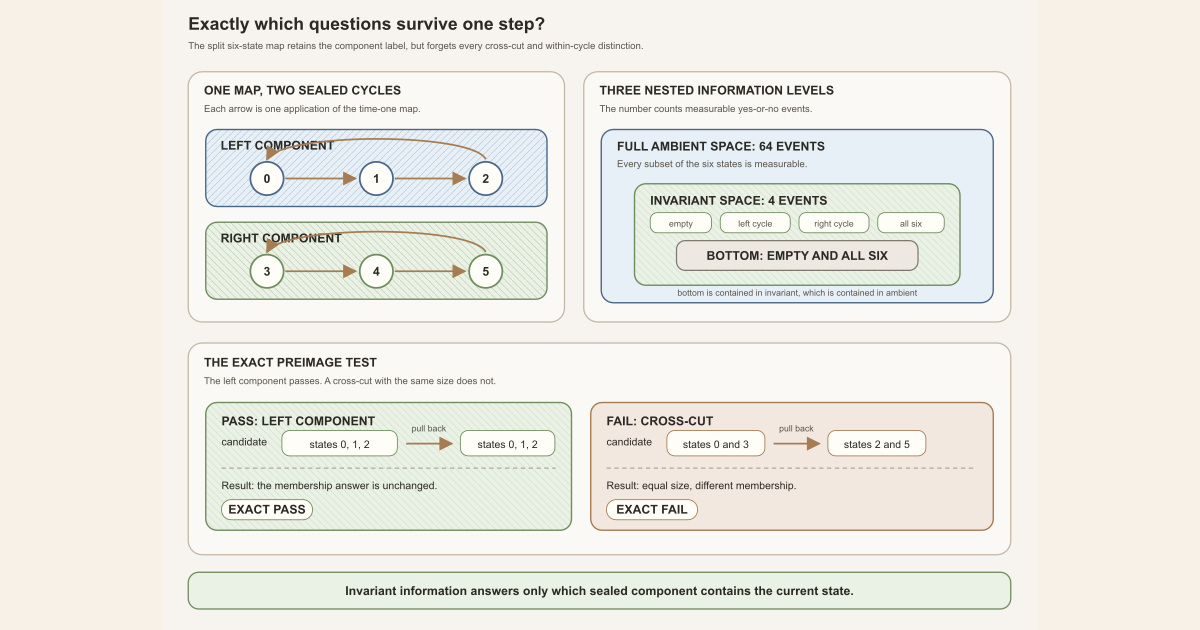
\[ \Omega=\{0,1,2,3,4,5\}. \]An event is a subset of \(\Omega\), a yes-or-no question about the current state. Declare every subset measurable, and give each state probability \(1/6\). That uniform probability measure will matter when we compare null sets; enumerating invariant events needs only the map and the measurable subsets. There are
\[ 2^6=64 \]such events: each of the six states can independently be included or excluded. Those \(64\) events form the full ambient sigma algebra \(\mathcal B\). A sigma algebra is a collection of events containing the empty event and closed under complements and countable unions. The measurable-space entry develops those closure rules from the beginning.
Now split the dynamics into two three-state cycles:
\[ \begin{aligned} T(0)&=1,&T(1)&=2,&T(2)&=0,\\ T(3)&=4,&T(4)&=5,&T(5)&=3. \end{aligned} \]Call the two components
\[ L=\{0,1,2\}, \qquad R=\{3,4,5\}. \]The preimage of an event \(S\) is
\[ T^{-1}(S)=\{x\in\Omega:T(x)\in S\}. \]This notation does not ask for an inverse function. It asks which starting states land in \(S\) after one step.
For the left component,
\[ T^{-1}(L)=\{0,1,2\}=L. \]The same calculation gives \(T^{-1}(R)=R\). The empty event and the whole space are also unchanged by preimage. Therefore these four events survive:
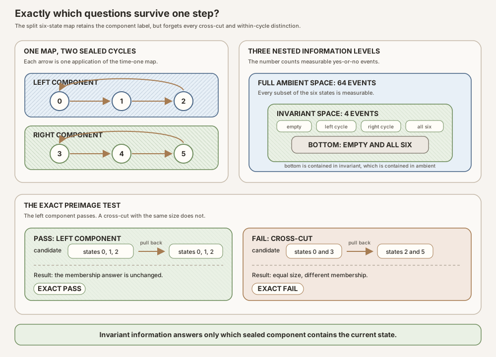
\[ \boxed{ \mathcal I_T =\{\varnothing,L,R,\Omega\}. } \]They are the complete invariant sigma algebra for this map. To see why the list is complete, suppose an invariant event contains state \(0\). Exact invariance says membership at \(x\) agrees with membership at \(T(x)\), so the event must also contain \(1\), then \(2\), then the whole left cycle. The same argument independently includes either all or none of the right cycle. There are two choices for each cycle, hence \(2^2=4\) invariant events.
Compare those four events with the smallest possible sigma algebra,
\[ \bot=\{\varnothing,\Omega\}. \]Lean calls this the bottom measurable space; probability texts often call it the trivial sigma algebra. In this example the three levels are strict:
\[ \{\varnothing,\Omega\} \subsetneq \{\varnothing,L,R,\Omega\} \subsetneq \mathcal P(\Omega), \]with \(2\), \(4\), and \(64\) events respectively. Here \(\mathcal P(\Omega)\) is the power set, meaning the collection of every subset of \(\Omega\).
The two-point event \(Q=\{0,3\}\) is a quick non-example:
\[ T^{-1}(Q)=\{2,5\}\ne\{0,3\}=Q. \]Having the same number of points is irrelevant. The actual membership question must remain unchanged.
The general definition
Let \((\Omega,\mathcal B)\) be a measurable space and let \(T:\Omega\to\Omega\) be any self-map. The invariant sigma algebra is
\[ \boxed{ \mathcal I_T =\{S\in\mathcal B:T^{-1}(S)=S\}. } \]Read the two gates separately:
- \(S\in\mathcal B\) says that \(S\) is an ambient measurable event.
- \(T^{-1}(S)=S\) is literal equality of ordinary sets.
The collection is itself a sigma algebra. Preimage fixes the empty set and the whole space, commutes with complement, and commutes with countable union:
\[ T^{-1}(S^{\mathsf c})=(T^{-1}S)^{\mathsf c}, \qquad T^{-1}\!\left(\bigcup_{j=0}^{\infty}S_j\right) =\bigcup_{j=0}^{\infty}T^{-1}(S_j). \]Ambient measurability is also preserved by the sigma-algebra closure rules. These facts prove closure of \(\mathcal I_T\).
No measure is needed to form this collection, and Mathlib’s definition does not require \(T\) to be measurable. Those hypotheses enter later when one transports integrals or proves an ergodic theorem. The raw definition is set-theoretic.
Full, invariant, and bottom information are different
The invariant sigma algebra can sit anywhere between the bottom and ambient measurable spaces:
\[ \bot\le \mathcal I_T\le\mathcal B. \]For measurable spaces, \(\mathcal A\le\mathcal B\) means every \(\mathcal A\)-measurable event is also \(\mathcal B\)-measurable. It is an information ordering: the larger sigma algebra can answer at least as many measurable yes-or-no questions.
The same six-state space gives three exact cases:
| Time-one map | Exactly invariant events | Invariant sigma algebra |
|---|---|---|
| Identity map | Every one of the \(64\) events | Full ambient space |
| One six-cycle | Only \(\varnothing\) and \(\Omega\) | Bottom space |
| Two three-cycles | \(\varnothing,L,R,\Omega\) | Strictly between them |
For the identity map, no membership answer ever changes. For one six-cycle, one included state forces inclusion of all six. For the split map, only the component label survives. This is the information that a conditional expectation onto \(\mathcal I_T\) is allowed to retain.
In Lean: membership means two exact tests
MeasurableSet[MeasurableSpace.invariants T] S ↔ MeasurableSet S ∧ T ⁻¹' S = SMeasurableSpace.invariants Tis the new measurable-space structure built from the self-mapT.- Square brackets in
MeasurableSet[… ] Sselect the measurable space against whichSis tested. - The ordinary
MeasurableSet Son the right uses the ambient measurable space already attached to the state type. ∧means both claims are required.T ⁻¹’ Sis Lean’s set-preimage notation.=means exact set equality. No measure and no almost-everywhere relation is hidden in the token.
The pinned Mathlib definition packages the same conjunction directly:
def MeasurableSpace.invariants
    [m : MeasurableSpace Ω] (T : Ω → Ω) : MeasurableSpace Ω :=
  { m ⊓ ⟨fun S ↦ T ⁻¹' S = S, by simp, by simp,
      fun F hF ↦ by simp [hF]⟩ with
    MeasurableSet' := fun S ↦ MeasurableSet[m] S ∧ T ⁻¹' S = S }
The operational theorem is definitionally exact:
theorem MeasurableSpace.measurableSet_invariants :
    MeasurableSet[MeasurableSpace.invariants T] S ↔
      MeasurableSet S ∧ T ⁻¹' S = S
The expression m ⊓ … intersects the ambient measurable space
with the preimage-fixed collection. A reader normally uses
measurableSet_invariants rather than unfolding this constructor.
Mathlib also records the ambient inclusion:
MeasurableSpace.invariants_le T :
  MeasurableSpace.invariants T ≤ inferInstance
It does not assert equality with the ambient space or with bottom. The map determines where the invariant sigma algebra lies between those extremes.
In Lean: invariant-measurable functions
A real-valued measurable function \(g:\Omega\to\mathbb R\) is measurable from \(\mathcal I_T\) when the inverse image of every Borel-measurable set of real numbers is an invariant event. The Borel sets are the standard measurable subsets of the real line generated by its open intervals. Mathlib’s exact interface is
Measurable[MeasurableSpace.invariants T] g ↔
  Measurable g ∧
    ∀ U, MeasurableSet U → (g ∘ T) ⁻¹' U = g ⁻¹' U
For a target whose singleton sets are measurable, including \(\mathbb R\), this forces pointwise function invariance.
MeasurableSpace.comp_eq_of_measurable_invariants hghg : Measurable[MeasurableSpace.invariants T] gis the input measurability proof.g ∘ Tis function composition; atωit reduces tog (T ω).comp_eq_of_measurable_invariantsuses measurable singleton fibers to turn equality of all measurable preimages into equality of values.- The returned equality is pointwise. It is stronger than
g ∘ T =ᵐ[μ] g, which would permit a null exceptional set.
In the split example, such a function may use one value on \(L\) and another on \(R\). Invariance means constant along each orbit component, not globally constant. Global almost-everywhere constancy needs the additional ergodicity hypothesis.
One-step invariance also implies invariance under every iterate:
MeasurableSpace.le_invariants_iterate T nT^[n]is Lean’s function-iterate notation for \(T^n\).≤compares measurable spaces by inclusion of their measurable events.- The theorem points only from one-step invariance to iterate invariance.
The reverse inclusion can fail. For the one six-cycle, \(T^2\) has two three-cycles, so it retains more events than \(T\). Equality would erase that periodic information.
Strict invariance is not invariance modulo null sets
Once a measure \(\mu\) is present, a second convention calls \(S\) invariant when its one-step preimage differs from it only on a null set :
\[ \mu\bigl(T^{-1}(S)\mathbin{\triangle}S\bigr)=0. \]The symmetric difference \(A\mathbin{\triangle}B\) contains the points that
belong to exactly one of \(A\) and \(B\). This is invariance modulo null
sets. It depends on \(\mu\); Mathlib’s
MeasurableSpace.invariants T does not.
The six-state uniform example hides the distinction because every state has positive probability \(1/6\). Its only null event is empty, so equality modulo null sets reduces to literal equality there.
A two-state example exposes the gap. Let \(\Omega=\{p,q\}\), put all probability mass at \(p\), and let \(T\) send both states to \(p\). This map preserves that Dirac probability measure. For \(S=\{q\}\),
\[ T^{-1}(S)=\varnothing\ne S, \qquad T^{-1}(S)\mathbin{\triangle}S=\{q\}, \qquad \mu(\{q\})=0. \]Thus \(S\) is invariant modulo null sets but is absent from Mathlib’s exact invariant sigma algebra. Exact invariance always implies modulo-null invariance. This two-state system is a counterexample to the converse, even among measure-preserving probability systems.
This distinction also separates two statements that sound similar:
- \(\mathcal I_T=\bot\) says that the only literal invariant measurable events are empty and full.
- Ergodicity says invariant measurable events are empty or full after null sets are ignored.
The first is stronger when nonempty null sets exist. An ergodic system need not have its exact invariant sigma algebra definitionally equal to bottom. For a concrete boundary, keep the same two-state Dirac probability but use the identity map. Every event is then exactly invariant, so the exact invariant sigma algebra is the full four-event ambient space. Nevertheless each event is null or conull because only \(p\) carries mass. The identity system is ergodic for this concentrated measure even though its exact invariant sigma algebra is not bottom.
Why the project uses the exact field
Random-matrix-theory milestone 27 (RMT-27) identifies finite-measure Birkhoff
limits with conditional expectation onto
MeasurableSpace.invariants T. Conditional expectations are unique
only
almost everywhere
, but the sigma
algebra supplied to that construction is still Mathlib’s exact field.
The project first defines one total real-valued representative
birkhoffLimit T f. Where finite
Birkhoff averages
converge, it selects their
limit; elsewhere it uses a fixed fallback. The theorem
birkhoffLimit_apply_base proves the ordinary pointwise identity
on both branches. Ambient measurability plus that literal invariance lets
measurable_birkhoffLimit_invariants place the chosen representative
in the exact invariant sigma algebra.
Under finite total measure, a measure-preserving map , and integrability of the observable, the final theorem proves almost-everywhere convergence to
μ[f | MeasurableSpace.invariants T]
It does not identify the exact field with a completed modulo-null field. It does not need to: the proof constructs the exact representative and applies conditional-expectation uniqueness for that exact sub-sigma algebra.
A tiny standalone Lean worksheet a human can type
Standalone tutorial. This file enumerates all \(64\) finite events and filters the four that pass the split map’s exact preimage test. It recreates finite Boolean set membership; it does not define Mathlib measurable spaces, measures, null sets, or conditional expectation.
Save it as InvariantSigmaFiniteScratch.lean:
import Std

def states : List Nat :=
  List.range 6

def splitCycles (x : Nat) : Nat :=
  if x < 3 then
    (x + 1) % 3
  else
    3 + (x - 3 + 1) % 3

def subsets : List (List Nat) :=
  states.foldr
    (fun x acc => acc ++ acc.map (fun event => x :: event))
    [[]]

def preimage (T : Nat → Nat) (event : List Nat) : List Nat :=
  states.filter fun x => event.contains (T x)

def invariant (T : Nat → Nat) (event : List Nat) : Bool :=
  preimage T event == event

def invariantEvents (T : Nat → Nat) : List (List Nat) :=
  subsets.filter fun event => invariant T event

#eval subsets.length
#eval invariantEvents splitCycles
#eval preimage splitCycles [0, 3]

example : subsets.length = 64 := by decide

example : invariantEvents splitCycles =
    [[], [3, 4, 5], [0, 1, 2], [0, 1, 2, 3, 4, 5]] := by
  decide

example : preimage splitCycles [0, 3] = [2, 5] := by decide
From the directory containing the file, type:
source "$HOME/.elan/env"
elan run leanprover/lean4:v4.32.0 lean InvariantSigmaFiniteScratch.lean
This exact worksheet was executed successfully with the pinned Lean 4.32.0 compiler and printed:
64
[[], [3, 4, 5], [0, 1, 2], [0, 1, 2, 3, 4, 5]]
[2, 5]
This command is suitable for an ordinary Mac or Linux machine because the
worksheet imports only Std. The worksheet is a finite audit of the
running example, not a proof of Mathlib’s general measure-theoretic interface,
and it does not load the project or Mathlib.
Try the exact declarations in the project
Full project check. This uses the repository’s pinned Lean and Mathlib dependencies and may require substantial disk space and memory. Create a temporary project worksheet containing:
import NonlinearDynamics.Random.RandomCocycles.PointwiseBirkhoffLimit

open MeasureTheory Set Filter Function
open NonlinearDynamics.Random.RandomCocycles

universe uΩ

variable {Ω : Type uΩ} [MeasurableSpace Ω]
variable {T : Ω → Ω} {S : Set Ω} {g : Ω → ℝ}
variable (hg : Measurable[MeasurableSpace.invariants T] g)

#check MeasurableSpace.invariants T
#check MeasurableSpace.measurableSet_invariants (f := T) (s := S)
#check MeasurableSpace.invariants_id (α := Ω)
#check MeasurableSpace.invariants_le T
#check MeasurableSpace.measurable_invariants_dom (f := T) (g := g)
#check MeasurableSpace.comp_eq_of_measurable_invariants hg
#check MeasurableSpace.le_invariants_iterate T 2
#check birkhoffLimit_apply_base
#check measurable_birkhoffLimit_invariants
#check setIntegral_orbit_iterate_eq
#check setIntegral_birkhoffLimit_eq
#check ae_tendsto_birkhoffAverage_condExp
Each #check asks the pinned elaborator for an exact declaration
type. The full-project command below checks the authoritative RMT-27 module with the
repository’s pinned dependencies installed.
cd formalization
lake env lean -DwarningAsError=true NonlinearDynamics/Random/RandomCocycles/PointwiseBirkhoffLimit.lean
Resource note: this exact file uses the repository's
pinned Lean and Mathlib dependencies. Initial project setup can require
substantial disk space and build time. For a lightweight first step on
macOS or Linux, use the page's standalone Lean-core or Std
tutorial.
Boundaries and nonclaims
- No measure is built into the definition. A measure enters only when a theorem asks about null sets, integrals, probability, or preservation.
- No inverse map is required. Set preimages exist for every function, including noninjective and nonsurjective maps.
- Invariant does not mean globally constant. A function may use different values on different invariant components, as the split example shows.
- Ergodicity is additional. It trivializes invariant information modulo null sets; it does not generally make the exact sigma algebra literally bottom.
- One-step and iterate invariance differ. A powered map can retain periodic phase information that one step does not.
- The sigma algebra proves no convergence by itself. Birkhoff convergence also needs analytic and measure-preserving hypotheses.
- No completion is implicit. The exact Mathlib field and a completed modulo-null invariant field must not be silently identified.
This entry does not construct an ergodic-component quotient, prove mixing, prove independence, or establish a Lyapunov exponent or an Oseledets splitting.
Where to continue
Identifying the Finite-Measure Birkhoff Limit in Lean maps RMT-27’s exact representative, invariant-set integral identities, and conditional-expectation endpoint to checked source.
Birkhoff Limits, Invariant Sigma Algebras, and Conditional Expectation builds the full proof architecture. The ergodicity entry compares the one-cycle and split-cycle systems under the same uniform probability. The Koopman operator entry develops the function-level pullback \(g\mapsto g\circ T\).
References
Mathlib contributors. Exact invariant measurable spaces, Mathlib 4.32.0 at pinned commit 81a5d257.