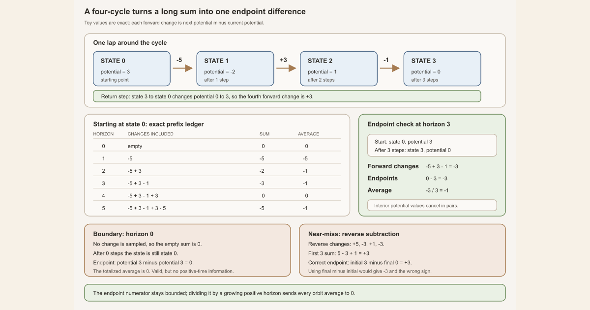
Start with four states and a map \(T\) that moves around one cycle:
\[ 0\xrightarrow{T}1\xrightarrow{T}2\xrightarrow{T}3 \xrightarrow{T}0. \]A potential assigns a number to each state. In this example let
\[ u(0)=3,\qquad u(1)=-2,\qquad u(2)=1,\qquad u(3)=0. \]The forward one-step change is “next potential minus current potential”:
\[ d(x)=u(Tx)-u(x). \]Compute it once at every state. Nothing is hidden in the notation:
| current state \(x\) | next state \(Tx\) | current \(u(x)\) | next \(u(Tx)\) | change \(d(x)\) |
|---|---|---|---|---|
| \(0\) | \(1\) | \(3\) | \(-2\) | \(-2-3=-5\) |
| \(1\) | \(2\) | \(-2\) | \(1\) | \(1-(-2)=3\) |
| \(2\) | \(3\) | \(1\) | \(0\) | \(0-1=-1\) |
| \(3\) | \(0\) | \(0\) | \(3\) | \(3-0=3\) |
Starting at state \(0\), the changes therefore repeat as
\[ -5,\ 3,\ -1,\ 3,\ -5,\ldots . \]A horizon \(n\) includes the readings at indices \(0,\ldots,n-1\). The following ledger computes every partial sum and average that will be used on this page:
| horizon \(n\) | changes included | partial sum \(S_nd(0)\) | totalized average \(A_nd(0)\) |
|---|---|---|---|
| \(0\) | empty sum | \(0\) | \(0\) |
| \(1\) | \(-5\) | \(-5\) | \(-5\) |
| \(2\) | \(-5+3\) | \(-2\) | \(-1\) |
| \(3\) | \(-5+3-1\) | \(-3\) | \(-1\) |
| \(4\) | \(-5+3-1+3\) | \(0\) | \(0\) |
| \(5\) | \(-5+3-1+3-5\) | \(-5\) | \(-1\) |
At horizon \(3\), the state reached after the three sampled changes is state \(3\). The entire sum is already the final potential minus the initial one:
\[ S_3d(0)=-5+3-1=-3=u(3)-u(0)=0-3. \]The intermediate values \(-2\) and \(1\) have disappeared. Each entered once with a plus sign and once with a minus sign. Dividing the endpoint difference by \(3\) gives \(A_3d(0)=-3/3=-1\).
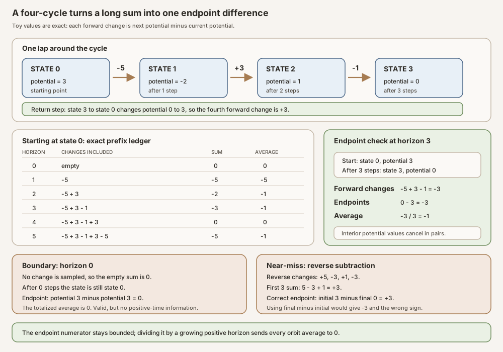
This example contains the whole finite algebra of a Koopman coboundary. The general definition explains why the same cancellation happens on every orbit, not just on a four-cycle.
From one-step change to Koopman coboundary
Let \(\Omega\) be any state space, let \(T:\Omega\to\Omega\) be any map, and let \(u:\Omega\to\mathbb R\) be a real-valued potential. The Koopman operator pulls an observable back along the dynamics:
\[ U_Tu=u\circ T, \qquad (U_Tu)(\omega)=u(T\omega). \]The project’s forward Koopman coboundary is
\[ d=(U_T-I)u, \qquad d(\omega)=u(T\omega)-u(\omega), \]where \(I\) is the identity operator. The word potential means the generating function \(u\). It does not mean physical energy unless a model supplies that extra interpretation.
This raw definition needs no measurable space, measure, probability, or inverse map. Koopman’s original composition-operator viewpoint arose in a Hilbert-space treatment of Hamiltonian systems (Koopman, 1931), but the finite identity here applies to an arbitrary self-map.
The endpoint telescope, one cancellation at a time
The iterate \(T^j\omega\) is the state reached after applying \(T\) exactly \(j\) times. Evaluate the coboundary at that state:
\[ d(T^j\omega) {} = u(T^{j+1}\omega)-u(T^j\omega). \]For a positive natural horizon \(n\), the Birkhoff sum expands as
\[ \begin{aligned} S_nd(\omega) &=\sum_{j=0}^{n-1}d(T^j\omega)\\ &=\bigl(u(T\omega)-u(\omega)\bigr) +\bigl(u(T^2\omega)-u(T\omega)\bigr)+\cdots\\ &\phantom{{}={}} +\bigl(u(T^n\omega)-u(T^{n-1}\omega)\bigr)\\ &=u(T^n\omega)-u(\omega). \end{aligned} \]Every interior potential appears once positively and once negatively. This is a telescoping sum: cancellation collapses a long chain to two endpoints.
Mathlib’s Birkhoff average is totalized at every natural horizon:
\[ A_nd(\omega) {} = (n:\mathbb R)^{-1}\bigl(u(T^n\omega)-u(\omega)\bigr). \]For \(n\gt0\), the scalar inverse is ordinary division by \(n\). At \(n=0\), the Birkhoff sum is empty, \(T^0\omega=\omega\), and the endpoint difference is zero. Lean’s real inverse also has \(0^{-1}=0\). Both sides are therefore zero. The formula is valid at horizon zero, but it is the vacuous equality \(0=0\), not a positive-time averaging fact.
Why bounded potentials force the averages to zero
Suppose \(u\) has bounded range. For a real-valued function, one sufficient way to state this is that some number \(M\ge0\) satisfies
\[ |u(\omega)|\le M \quad\text{for every }\omega\in\Omega. \]Then, for every positive \(n\),
\[ \begin{aligned} |A_nd(\omega)| &=\frac{|u(T^n\omega)-u(\omega)|}{n}\\ &\le\frac{|u(T^n\omega)|+|u(\omega)|}{n}\\ &\le\frac{2M}{n} \longrightarrow0. \end{aligned} \]The conclusion holds at every starting state. It needs neither a measure nor measure preservation , finite mass, probability normalization, ergodicity, or invertibility.
In the four-cycle, the endpoint numerator is always one of \(0,-5,-2,-3\). Its absolute value is at most \(5\), so the sharper example-specific estimate is
\[ |A_nd(0)|\le\frac5n \quad(n\gt0). \]The averages in the ledger are not monotone, but monotonicity is irrelevant: a bounded numerator divided by a growing positive horizon still tends to zero.
Near-miss: reversing the subtraction reverses the endpoint
Some books use the opposite convention
\[ \widetilde d=(I-U_T)u, \qquad \widetilde d(x)=u(x)-u(Tx)=-d(x). \]For the same four-cycle, the reverse-convention values are
\[ 5,\ -3,\ 1,\ -3. \]At horizon \(3\), they sum to
\[ 5-3+1=3=u(0)-u(3). \]The common mistake is to use these reverse changes but retain the forward endpoint \(u(T^3 0)-u(0)=-3\). That would assert \(3=-3\). Both conventions telescope, but they telescope in opposite directions. The zero-horizon case cannot detect this bug because both endpoint orders reduce to zero there. RMT-25 consistently uses \(U_T-I\).
Where measure preservation and real \(L^2\) enter
The raw telescope is pointwise algebra. A separate analytic construction begins when \(\Omega\) carries a measure \(\mu\) and \(T\) preserves it. A real \(L^2(\mu)\) vector is a square-integrable real function considered up to almost-everywhere equality . In other words, two representatives define the same vector when they disagree only on a null set .
Measure preservation makes composition by \(T\) a continuous linear contraction on \(L^2(\mu)\). The project therefore defines
\[ C_T=U_T-I:L^2(\mu)\to L^2(\mu). \]This bundled operator is koopmanCoboundaryL2. The
measure-preserving hypothesis is needed here because the operator acts on
almost-everywhere equivalence classes. It was not needed for the raw
function \(x\mapsto u(Tx)-u(x)\).
Why simple potentials produce a dense pointwise-good core
A simple function takes only finitely many values. Any chosen finite-range real representative is bounded, so its raw forward coboundary has pointwise Birkhoff averages tending to zero. Mathlib supplies dense simple vectors in real \(L^2\) (pinned simple-function implementation).
RMT-25 names the coboundaries generated by those vectors:
\[ \mathcal C_{\mathrm{simp}} {} = \{C_Tu:u\text{ is a simple }L^2\text{ vector}\}. \]Let \(K=\operatorname{Fix}(U_T)\), the closed subspace of vectors unchanged by Koopman composition. The checked Hilbert-space geometry gives the one-sided inclusion
\[ K^\perp \subseteq \overline{\operatorname{range}(C_T)}. \]Here \(K^\perp\) is the orthogonal complement of the fixed subspace and the bar denotes topological closure. The historical projection argument goes back to von Neumann’s mean theorem (von Neumann, 1932); RMT-25 uses Mathlib’s closure-of-range implementation (pinned mean-ergodic source).
Continuity of \(C_T\) and density of simple vectors strengthen the usable conclusion: every vector in \(K^\perp\) can be approximated by members of \(\mathcal C_{\mathrm{simp}}\). Orthogonal projection splits an arbitrary \(f\in L^2\) into a fixed part and a perpendicular remainder. Consequently,
\[ \{h+c:h\in K,\ c\in\mathcal C_{\mathrm{simp}}\} \]is dense in real \(L^2\).
There is an essential representative boundary. Equality in \(L^2\) means almost-everywhere equality, not pointwise equality at every state. The chosen representative of \(C_Tu\) is only almost everywhere equal to the raw function \(u\circ T-u\). RMT-25 transports that equality through the Birkhoff convergence event and intersects the countably many representative equalities needed for fixed vectors. It does not silently substitute one representative for another at every point.
The final core theorem is therefore an almost-everywhere statement about chosen representatives. It does not say that every representative of every \(L^2\) coboundary converges pointwise. Nor does density alone promote the good-core result to a full pointwise theorem. The later maximal-inequality argument makes convergence stable under \(L^1\) approximation, following the route highlighted by Keane and Petersen (Keane and Petersen, 2006).
Assumption ladder
| Claim | Assumptions actually used | Claim not obtained |
|---|---|---|
| Four-cycle arithmetic | the displayed map and four potential values | a result for every system |
| Raw endpoint telescope | any self-map \(T\), real potential \(u\), state, and finite horizon | measurability or a limit theorem |
| Pointwise zero limit | bounded range of \(u\) | a statement about every unbounded potential |
| Real \(L^2\) coboundary operator | MeasurePreserving T μ μ | a canonical pointwise representative |
| Dense fixed-plus-simple-coboundary core | measure preservation and real Hilbert-space exponent \(2\) | exact representation of every vector as one coboundary |
| Almost-everywhere good-core theorem | measure preservation plus representative bookkeeping | full-sequence pointwise convergence for arbitrary \(L^2\) data |
Finite total mass, probability normalization, ergodicity, injectivity, surjectivity, and invertibility are absent from every RMT-25 declaration named on this page.
In Lean: the sign convention in three languages
fun x ↦ u (T x) - u xfun x ↦starts an anonymous function with inputx.T xis the state after one step.u (T x)reads the potential at that next state.- u xsubtracts the current potential. Reversing these two terms changes the convention.- No measure or \(L^2\) type appears in this raw expression.
In Lean: the all-horizon endpoint identity
birkhoffAverage_forwardCoboundary u n ωbirkhoffAverage ℝ Tmeans the real Birkhoff average along the mapT.fun x ↦ u (T x) - u xis the forward coboundary observable.n : ℕis the number of sampled changes.T^[n]is Lean’s notation for the \(n\)-fold iterate ofT.(n : ℝ)⁻¹casts the natural horizon to a real number and then takes its totalized inverse.•is scalar multiplication. For reals it gives the same value as multiplication by \(1/n\) when \(n\gt0\).- The proof term includes \(n=0\); its zero case is valid but vacuous.
The exact project theorem has this shape:
theorem birkhoffAverage_forwardCoboundary (u : Ω → ℝ)
    (n : ℕ) (ω : Ω) :
    birkhoffAverage ℝ T (fun x ↦ u (T x) - u x) n ω =
      (n : ℝ)⁻¹ • (u (T^[n] ω) - u ω)
In Lean: bounded range gives pointwise convergence
tendsto_birkhoffAverage_forwardCoboundary u hu ωhu : Bornology.IsBounded (Set.range u)is the bounded-range hypothesis.Tendstois Lean’s filter-based statement of convergence.atTopsends the natural horizon toward infinity.nhds 0is the neighborhood filter of the real number zero.ωis fixed, so the conclusion is pointwise at that starting state, not merely almost everywhere.
The theorem concludes:
Tendsto (fun n ↦ birkhoffAverage ℝ T
  (fun x ↦ u (T x) - u x) n ω) atTop (nhds 0)
A tiny standalone Lean worksheet a human can type
Standalone tutorial. This file computes only the finite four-cycle arithmetic. It does not import Mathlib, prove the general telescope, construct an \(L^2\) operator, or check the project module.
Save the following as KoopmanCoboundaryTutorial.lean:
import Std

inductive CycleState where
  | s0 | s1 | s2 | s3
deriving Repr, DecidableEq

def step : CycleState → CycleState
  | .s0 => .s1
  | .s1 => .s2
  | .s2 => .s3
  | .s3 => .s0

def potential : CycleState → Int
  | .s0 => 3
  | .s1 => -2
  | .s2 => 1
  | .s3 => 0

def iterate : Nat → CycleState → CycleState
  | 0, x => x
  | n + 1, x => iterate n (step x)

def forwardChange (x : CycleState) : Int :=
  potential (step x) - potential x

def reverseChange (x : CycleState) : Int :=
  potential x - potential (step x)

def orbitSum (g : CycleState → Int) : Nat → CycleState → Int
  | 0, _ => 0
  | n + 1, x => orbitSum g n x + g (iterate n x)

def endpointDifference (n : Nat) (x : CycleState) : Int :=
  potential (iterate n x) - potential x

def totalizedAverage (n : Nat) (x : CycleState) : Rat :=
  match n with
  | 0 => 0
  | n + 1 => (orbitSum forwardChange (n + 1) x : Rat) / (n + 1 : Rat)

def states : List CycleState := [.s0, .s1, .s2, .s3]

#eval states.map potential
#eval states.map forwardChange
#eval (List.range 6).map (fun n => orbitSum forwardChange n .s0)
#eval (List.range 6).map (fun n => totalizedAverage n .s0)

example : states.map forwardChange = [-5, 3, -1, 3] := by
  decide

example : (List.range 6).map (fun n => orbitSum forwardChange n .s0) =
    [0, -5, -2, -3, 0, -5] := by
  decide

example : (List.range 6).map (fun n => totalizedAverage n .s0) =
    [(0 : Rat), -5, -1, -1, 0, -1] := by
  native_decide

example : orbitSum forwardChange 3 .s0 = endpointDifference 3 .s0 := by
  decide

example : orbitSum reverseChange 3 .s0 = 3 := by
  decide

example : endpointDifference 3 .s0 = -3 := by
  decide
From the directory containing the file, type:
source "$HOME/.elan/env"
elan run leanprover/lean4:v4.32.0 lean KoopmanCoboundaryTutorial.lean
This exact worksheet was executed successfully with Lean 4.32.0 while editing
this page. It printed potentials [3, -2, 1, 0], forward changes
[-5, 3, -1, 3], partial sums
[0, -5, -2, -3, 0, -5], and totalized averages
[0, -5, -1, -1, 0, -1]. This command is suitable for an ordinary
Mac or Linux machine because the worksheet imports only Std and
has a finite state space.
Try the exact declarations in the project
Full project check. This uses the repository’s pinned Lean and Mathlib dependencies and may require substantial disk space and memory. Place this query in a temporary project scratch file:
import NonlinearDynamics.Random.RandomCocycles.KoopmanL2Mean

open MeasureTheory Set Filter Function
open NonlinearDynamics.Random.RandomCocycles

#check birkhoffAverage_forwardCoboundary
#check tendsto_birkhoffAverage_forwardCoboundary
#check koopmanL2
#check koopmanCoboundaryL2
#check simpleKoopmanCoboundarySetL2
#check fixedOrthogonal_le_closure_range_koopmanL2
#check fixedOrthogonal_subset_closure_simpleKoopmanCoboundarySetL2
#check dense_fixedPlusSimpleCoboundarySetL2
#check ae_mem_birkhoffConvergenceSet_of_mem_simpleKoopmanCoboundarySetL2
#check ae_mem_birkhoffConvergenceSet_of_mem_fixedPlusSimpleCoboundarySetL2

#print birkhoffAverage_forwardCoboundary
Each #check asks the pinned elaborator for the exact declaration
type. #print also shows the theorem body and inferred parameters.
The full-project command printed below checks the authoritative RMT-25 source
file. It is separate from the standalone tutorial and uses the repository’s
pinned dependencies.
cd formalization
lake env lean -DwarningAsError=true NonlinearDynamics/Random/RandomCocycles/KoopmanL2Mean.lean
Resource note: this exact file uses the repository's
pinned Lean and Mathlib dependencies. Initial project setup can require
substantial disk space and build time. For a lightweight first step on
macOS or Linux, use the page's standalone Lean-core or Std
tutorial.
What this term does not claim
A Koopman coboundary does not by itself imply:
- that its generating \(L^2\) potential has an essentially bounded or canonical pointwise representative;
- pointwise convergence for every arbitrary representative of an \(L^2\) coboundary;
- that every vector orthogonal to the fixed space is an exact coboundary;
- equality between the fixed orthogonal complement and the exported closed range, beyond the checked one-sided inclusion;
- full-sequence pointwise convergence for every \(L^2\) or \(L^1\) observable;
- identification of the eventual limit with a conditional expectation;
- ergodicity, mixing, independence, or decay of correlations;
- a strong \(L^1\) maximal inequality;
- Kingman’s subadditive ergodic theorem; or
- a Lyapunov exponent or Oseledets splitting.
The exact finite telescope converts this particular class of observables into endpoint arithmetic. It is not a general pointwise ergodic theorem.
Where to continue
Mean Is Not Pointwise: Koopman Geometry, Coboundaries, and the Missing Maximal Step develops the Hilbert-space geometry, representative issues, and maximal-closure handoff as a textbook chapter.
Koopman L² Mean Convergence and a Dense Pointwise-Good Core in Lean maps RMT-25’s named declarations to the checked source and its proof architecture.
The Koopman operator entry develops the composition operator itself. The Birkhoff sum entry teaches the finite orbit sum and its horizon convention before any convergence theorem. The Birkhoff convergence event entry packages the set of starting points whose averages converge.
References
B. O. Koopman. Hamiltonian Systems and Transformation in Hilbert Space, Proceedings of the National Academy of Sciences 17(5), 315-318, 1931, DOI 10.1073/pnas.17.5.315. Pages 315-316 are the primary historical source for the composition-operator view underlying \(U_T-I\). RMT-25 uses a discrete real \(L^2\) specialization and does not inherit the paper’s invertible Hamiltonian setting.
John von Neumann. Proof of the Quasi-Ergodic Hypothesis, Proceedings of the National Academy of Sciences 18(1), 70-82, 1932, DOI 10.1073/pnas.18.1.70. Pages 72-74 give the historical Hilbert-space projection argument. It is lineage for the fixed-space and coboundary-range geometry, not the exact Mathlib theorem statement.
Michael Keane and Karl Petersen. Easy and Nearly Simultaneous Proofs of the Ergodic Theorem and Maximal Ergodic Theorem, Institute of Mathematical Statistics Lecture Notes-Monograph Series 48, 248-251, 2006, DOI 10.1214/074921706000000266. This primary proof source shows how a strengthened maximal estimate yields a pointwise ergodic theorem. It supports the missing-maximal-step comparison; RMT-25 itself supplies the dense core only.
Mathlib contributors. Density of simple functions in \(L^p\), with the pinned v4.32.0 representative and density implementation. The finite-range representative and dense embedding are the exact upstream interfaces used for the simple-coboundary core.
Mathlib contributors. Pinned von Neumann mean-ergodic implementation, Mathlib v4.32.0. Its closure-of-range and orthogonal-projection theory is the formal geometry specialized by RMT-25.
The exact upstream revision for both pinned Mathlib references is commit
81a5d257,
the version recorded in formalization/lake-manifest.json.