Koopman operator

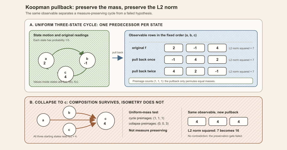
Start with three states and a clockwise update:

An observable is a function that assigns a readable number to each state. Choose

The Koopman operator does not move these three numbers directly. It asks, at each starting state, “where will the state go next, and what number does \(f\) read there?” Its defining rule is

Calculate all three values:

In the fixed order \((a,b,c)\), this is

The states move forward, while the table of values is pulled back to the starting states.

Pull back twice

Apply the same rule to the new observable:

Therefore

Following the state twice and then reading \(f\) is the same operation:

More generally, for every natural number \(n\),

Because this example is a three-cycle, \(T^3\) is the identity and \(U_T^3f=f\).

Check the square-integrable norm

Give each state probability \(1/3\). This uniform probability measure makes the cycle measure preserving: every state has exactly one predecessor, so the cycle only permutes three equal masses.

For a real observable \(g\), its squared \(L^2\) norm is the uniform average of its squared readings:

For the original observable,

The pulled-back values are a permutation of the same three readings, so

The second pullback has the same result:

Thus this finite calculation exhibits the isometry law

An isometry preserves distance from zero, equivalently the norm. It need not be onto.

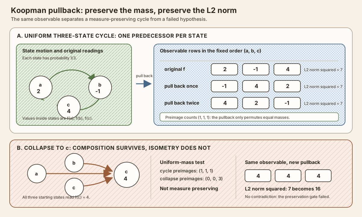
Near-miss: composition without measure preservation

Keep the same state space, uniform probability, and observable, but replace the cycle by the collapse map

This map is measurable on the finite space, but it does not preserve the uniform measure. For the one-point event \(A=\{c\}\),

Pointwise composition still makes sense:

But the norm calculation is now

Nothing has gone wrong with the definition \(U_Cf=f\circ C\). The isometry conclusion failed because its measure-preservation hypothesis failed. In the project, one cannot construct koopmanL2 hC for this uniform collapse without supplying the impossible certificate hC : MeasurePreserving C μ μ.

General definition

Let \(\Omega\) be a set of states equipped with a measurable space \(\Sigma\) and a measure \(\mu\). Let \(T:\Omega\to\Omega\) be a measurable function . For an observable \(f:\Omega\to\mathbb R\), define the pointwise composition operator by

The project fixes this forward-composition convention. Some sources for invertible dynamics use composition with \(T^{-1}\). That is a different operator, so the two conventions cannot be exchanged silently.

The name pullback describes the arrow reversal:

• the state arrow sends \(\omega\) forward to \(T\omega\); and
• the observable \(f\), which reads values at destination states, becomes the new observable \(f\circ T\) on starting states.

Evaluation closes the two descriptions into one equality:

Why the operator is linear

The state update \(T\) may be nonlinear. Linearity is instead a statement about the input observable. For real numbers \(\alpha,\beta\) and observables \(f,g\),

Therefore

For example, even when a state variable obeys the nonlinear update \(T(x)=x^2\), the rule \(U_Tf(x)=f(x^2)\) is linear in \(f\). This algebraic fact alone says nothing about whether a chosen measure is preserved.

From functions to real \(L^2\)

A real \(L^2(\mu)\) vector is not literally one function. It is an almost-everywhere equivalence class of measurable functions for which \(|f|^2\) is integrable . Two representatives describe the same vector when they differ only on a null set .

Suppose \(T\) is a measure-preserving transformation :

for every measurable event \(A\). Measure preservation does two jobs:

1. it transports null sets through preimages, so \([f\circ T]\) does not depend on the chosen representative \(f\); and
2. it gives the change-of-variables identity needed for the norm calculation.

The resulting operator on equivalence classes is

Its exact norm identity is

No finite-total-mass, probability, ergodicity, injectivity, surjectivity, or invertibility premise is needed for this real \(L^2\) composition isometry. The three-state example uses a probability so that every integral reduces to a finite weighted sum.

Isometry does not mean unitary equivalence

The project exposes the Koopman map as a continuous linear map and proves the assumption-safe operator-norm bound

It does not claim unconditional equality with one. Under the zero measure, real \(L^2\) is the trivial space and the operator norm is zero, even though every vector-level norm identity remains true.

Nor does an isometry have to be surjective. On one-sided fair coin sequences, let \(T\) discard the first bit. This shift preserves product probability. Every function in the range of \(U_T\) depends only on the tail, so the first-bit observable is not in the range, even modulo null sets. Thus measure-preserving composition can be isometric without being a unitary equivalence.

Why physicists and dynamicists use it

The state trajectory may follow a nonlinear law, but measurements still live in a vector space: observables can be added and scaled. Koopman composition uses that linear structure without assuming that the original state update is linear. Iteration produces

which records how one measurement changes as the state advances. Spectral and Hilbert-space tools can then study invariant observables and time averages. This viewpoint transfers observables into linear operator language. It does not turn the original nonlinear system into a finite-dimensional linear one, nor does it supply a tractable spectral computation.

Fixed observables and mean convergence

The fixed subspace is

Equality here is equality in \(L^2\), hence equality almost everywhere, not necessarily pointwise equality for every chosen representative.

Let \(P_K\) denote orthogonal projection onto \(K\). The project specializes Mathlib’s mean-ergodic theorem to prove

For the three-cycle, one complete operator average is

It is constant and therefore fixed. In this particular one-cycle model, the fixed vectors are precisely the constant functions. The general project theorem does not identify every fixed subspace with constants. That requires an additional ergodicity argument.

Norm convergence also does not by itself prove full-sequence pointwise convergence. The project first obtains an almost-everywhere convergent subsequence and develops a dense pointwise-good core using Koopman coboundaries . Later modules add maximal control to reach the pointwise Birkhoff theorem.

In Lean: apply the composition operator

koopmanL2 hT f = Lp.compMeasurePreserving T hT f

The source definition deliberately begins with a linear isometry and then drops only the extra packaging needed to expose a continuous linear map:

def koopmanL2 (hT : MeasurePreserving T μ μ) :
    Lp ℝ 2 μ →L[ℝ] Lp ℝ 2 μ :=
  (Lp.compMeasurePreservingₗᵢ ℝ T hT).toContinuousLinearMap

The arrow →L[ℝ] means a continuous real-linear map. The object compMeasurePreservingₗᵢ before conversion has the stronger linear-isometry type.

In Lean: preserve the \(L^2\) norm

Lp.norm_compMeasurePreserving f hT

The operator-level statement is intentionally weaker:

norm_koopmanL2_le hT

In Lean: iterate state motion and observable pullback together

iterate_koopmanL2_apply hT n f

Standalone tutorial

Standalone tutorial. This complete file reproduces the three-state cycle, both pullbacks, the uniform squared-norm numerators, and the non-preserving collapse. It imports Std, not Mathlib or this project.

Save it as KoopmanFiniteScratch.lean:

import Std

namespace KoopmanFiniteScratch

inductive State where
  | a | b | c
deriving Repr, DecidableEq

def points : List State := [.a, .b, .c]

def cycle : State → State
  | .a => .b
  | .b => .c
  | .c => .a

def collapse : State → State := fun _ => .c

def observable : State → Int
  | .a => 2
  | .b => -1
  | .c => 4

def pullback (T : State → State) (f : State → Int) : State → Int :=
  fun state => f (T state)

def values (f : State → Int) : List Int :=
  points.map f

def squaredMassNumerator (f : State → Int) : Int :=
  (values f).foldl (fun total value => total + value * value) 0

def preimageCount (T : State → State) (target : State) : Nat :=
  (points.filter fun source => decide (T source = target)).length

def preimageCounts (T : State → State) : List Nat :=
  points.map (preimageCount T)

#eval values observable
#eval values (pullback cycle observable)
#eval values (pullback cycle (pullback cycle observable))
#eval squaredMassNumerator observable
#eval squaredMassNumerator (pullback cycle observable)
#eval preimageCounts cycle
#eval preimageCounts collapse
#eval values (pullback collapse observable)
#eval squaredMassNumerator (pullback collapse observable)

example : values observable = [2, -1, 4] := by decide
example : values (pullback cycle observable) = [-1, 4, 2] := by decide
example : values (pullback cycle (pullback cycle observable)) =
    [4, 2, -1] := by decide
example : squaredMassNumerator observable = 21 := by decide
example : squaredMassNumerator (pullback cycle observable) = 21 := by decide
example : preimageCounts cycle = [1, 1, 1] := by decide
example : preimageCounts collapse = [0, 0, 3] := by decide
example : values (pullback collapse observable) = [4, 4, 4] := by decide
example : squaredMassNumerator (pullback collapse observable) = 48 := by decide

end KoopmanFiniteScratch

Run exactly this small file on macOS or Linux with the pinned compiler:

source "$HOME/.elan/env"
elan run leanprover/lean4:v4.32.0 lean KoopmanFiniteScratch.lean

The first three output rows should be [2, -1, 4], [-1, 4, 2], and [4, 2, -1]. The cycle has squared-mass numerator 21 before and after pullback, and division by the three equal masses gives squared \(L^2\) norm \(7\). The collapse has preimage counts [0, 0, 3], pulled-back values [4, 4, 4], and numerator 48, which gives squared norm \(16\).

This worksheet checks finite function composition and integer arithmetic. It does not instantiate Mathlib’s measure, \(L^2\), or continuous-linear-map interfaces. This exact worksheet was executed successfully with the pinned Lean 4.32.0 compiler.

Try the exact declarations in the project

import NonlinearDynamics.Random.RandomCocycles.KoopmanL2Mean

open MeasureTheory
open NonlinearDynamics.Random.RandomCocycles

#check koopmanL2
#check koopmanL2_apply
#check Lp.norm_compMeasurePreserving
#check iterate_koopmanL2_apply
#check norm_koopmanL2_le
#check koopmanFixedSubspaceL2
#check koopmanInvariantProjectionL2
#check tendsto_birkhoffAverage_koopmanL2_projection
#check exists_subsequence_ae_tendsto_birkhoffAverage_koopmanL2_projection

cd formalization
lake env lean -DwarningAsError=true NonlinearDynamics/Random/RandomCocycles/KoopmanL2Mean.lean

Boundary cases and common confusions

• Identity dynamics: if \(T\omega=\omega\), then \(U_Tf=f\) for every observable.
• Constant observable: if \(f\) has one value everywhere, then \(U_Tf=f\) for every state map, preserving or not.
• Non-preserving map: pointwise composition remains linear, but the chosen \(L^2(\mu)\) norm need not be preserved. The collapse example changes its square from \(7\) to \(16\).
• Zero measure: vector norms are still preserved, but the continuous linear operator norm is zero rather than one.
• Noninvertible preserving map: an isometric Koopman operator need not be onto. Measure preservation is not the same as bijectivity.
• Representatives: \((U_Tf)(\omega)=f(T\omega)\) is a pointwise formula for chosen representatives. The actual \(L^2\) object is an almost-everywhere equivalence class.
• Iteration order: the project uses forward composition \(U_Tf=f\circ T\), hence \(U_T^nf=f\circ T^n\).

What the term does not establish

A Koopman operator by itself does not prove:

• that the state update is linear, smooth, injective, surjective, or invertible;
• that the composition operator is a unitary equivalence;
• that its operator norm is exactly one on a degenerate measure space;
• that every fixed observable is constant;
• that the system is ergodic, mixing, chaotic, or independent;
• that finite averages converge pointwise along the full sequence;
• that the invariant projection is already identified as conditional expectation; or
• a Kingman theorem, Lyapunov exponent, Lyapunov spectrum, or Oseledets splitting.

RMT-25 constructs the real \(L^2\) operator, its fixed subspace, its orthogonal projection, and norm convergence of its finite means. The complete ascent is Mean Is Not Pointwise: Koopman Geometry, Coboundaries, and the Missing Maximal Step. The declaration-level account is Koopman L² Mean Convergence and a Dense Pointwise-Good Core in Lean.

Check your understanding

1. Starting from \(b\), what number does \(U_T^2f\) read in the three-cycle?
2. Why do the preimage counts \((1,1,1)\) certify uniform-mass preservation for a map on three points?
3. Recompute the collapse near-miss if every state is sent to \(a\) instead of \(c\). Does the norm grow or shrink?
4. Why can \(U_T\) be linear even when \(T\) is nonlinear?
5. Which hypothesis is used to turn \([f]\mapsto[f\circ T]\) into an isometry on \(L^2(\mu)\)?

References

B. O. Koopman. Hamiltonian Systems and Transformation in Hilbert Space, Proceedings of the National Academy of Sciences 17(5), 315-318, 1931, DOI 10.1073/pnas.17.5.315. Pages 315-316 construct composition operators for continuous-time Hamiltonian flows with an invariant positive density. That historical unitary setting is stronger than the project’s discrete, potentially noninvertible interface.

John von Neumann. Proof of the Quasi-Ergodic Hypothesis, Proceedings of the National Academy of Sciences 18(1), 70-82, 1932, DOI 10.1073/pnas.18.1.70. Pages 71-74 develop the Hilbert-norm projection form of mean convergence. The project uses Mathlib’s discrete contraction theorem rather than reproducing the original continuous-time spectral argument.

George D. Birkhoff. Proof of the Ergodic Theorem, Proceedings of the National Academy of Sciences 17(12), 656-660, 1931, DOI 10.1073/pnas.17.2.656. Page 656 separates convergence in the mean from the pointwise problem. The publisher displays the DOI segment 17.2 even though the bibliographic issue is 17(12).

Mathlib contributors. Von Neumann mean ergodic theorem, with the pinned v4.32.0 implementation. The theorem for a contracting continuous linear self-map is the upstream result specialized by RMT-25.

Mathlib contributors. Pinned measure-preserving \(L^p\) composition API, Mathlib v4.32.0. These declarations supply representative composition, the iterate law, exact norm preservation, and the linear isometry used by koopmanL2.

The exact upstream revision for both Mathlib references is commit 81a5d257, the revision pinned by formalization/lake-manifest.json.