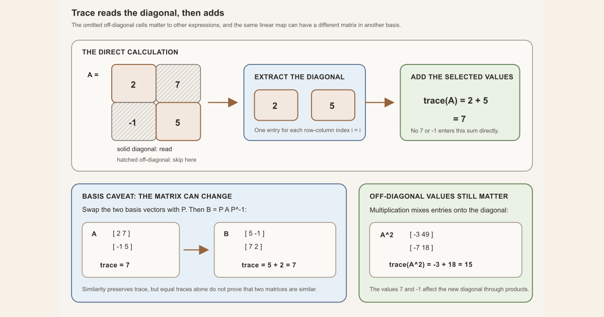
The trace of a finite square matrix is found by reading its main diagonal and adding those entries. It turns an entire matrix into one scalar.
Start with one 2 by 2 matrix
Take
\[ A= \begin{bmatrix} 2&7\\ -1&5 \end{bmatrix}. \]The main diagonal runs from the top-left entry to the bottom-right entry, so
\[ \operatorname{tr}(A)=2+5=7. \]The entries \(7\) and \(-1\) are off the main diagonal. They do not enter this particular sum directly. In general, for a square matrix whose rows and columns share the finite index set \(I\),
\[ \operatorname{tr}(A)=\sum_{i\in I}A_{ii}. \]
Why off-diagonal entries still matter
The phrase “trace ignores off-diagonal entries” is safe only for the direct calculation of \(\operatorname{tr}(A)\). Matrix multiplication mixes rows and columns. In this example,
\[ A^2 {} = \begin{bmatrix} -3&49\\ -7&18 \end{bmatrix}, \qquad \operatorname{tr}(A^2)=-3+18=15. \]The new top-left entry is
\[ (A^2)_{11}=2\cdot2+7\cdot(-1)=-3, \]so the old off-diagonal entries now influence a diagonal entry. This is why the trace-power observable \(\operatorname{tr}(A^k)\) contains more information than \(\operatorname{tr}(A)\) alone.
Why the trace is structural
The coordinate matrix of a linear operator changes when its basis changes. The individual diagonal entries can change too, but their sum does not. For the example, let
\[ P= \begin{bmatrix} 0&1\\ 1&0 \end{bmatrix}. \]This matrix swaps the two basis vectors and satisfies \(P^{-1}=P\). The similar matrix is
\[ B=PAP^{-1} {} = \begin{bmatrix} 5&-1\\ 7&2 \end{bmatrix}, \qquad \operatorname{tr}(B)=5+2=7. \]The general calculation uses cyclicity. For compatible finite square matrices,
\[ \operatorname{tr}(AB)=\operatorname{tr}(BA). \]If \(S\) is invertible, then
\[ \operatorname{tr}(SAS^{-1}) {} = \operatorname{tr}(AS^{-1}S) {} = \operatorname{tr}(A). \]Thus trace is a basis-independent feature of a finite-dimensional linear endomorphism, even though its coordinate formula is a diagonal sum. This is a specific similarity statement. It does not say that trace is unchanged under an arbitrary edit or rearrangement of matrix entries.
The converse is false: equal traces do not imply similarity. The zero matrix and
\[ N= \begin{bmatrix} 0&1\\ 0&0 \end{bmatrix} \]both have trace zero, but the nonzero matrix \(N\) cannot be similar to the zero matrix.
When \(H\) is Hermitian , its diagonal entries are real, so \(\operatorname{tr}(H)\) is real. From the spectral viewpoint, its eigenvalues are real and, with multiplicity, their sum equals the trace. That spectral statement uses additional finite-dimensional eigenvalue theory; it is not the definition of trace.
Trace as a random-matrix observable
For a finite random matrix \(X:\Omega\to\mathbb C^{n\times n}\), the trace becomes a scalar function of the outcome:
\[ \omega\longmapsto\operatorname{tr}(X(\omega)). \]The project proves this function is measurable whenever \(X\) is measurable. The proof expands trace into a finite sum of measurable diagonal coordinates. If one realization equals the example matrix \(A\), then the scalar observable returns seven on that outcome. A different realization can return a different number. Taking the trace pointwise does not take an expectation over outcomes.
In Lean
Lean writes the operation on one matrix as Matrix.trace A. The
project theorem connects the finite diagonal sum to probability by showing
that pointwise trace preserves measurability.
RandomMatrix.measurable_trace hX : Measurable fun ω ↦ Matrix.trace (X ω)Xis a square complexRandomMatrix Ω ι ι ℂ. Usingιfor both matrix indices is Lean’s version of “square.”[Fintype ι]tells Lean that the diagonal index set is finite, so its entries can be added with a finite sum.hX : Measurable Xis the hypothesis that the matrix-valued map is measurable.fun ω ↦ Matrix.trace (X ω)is an anonymous function: take an outcomeω, realizeX ω, and compute its trace.Measurablebefore that function is the conclusion. The colon in the Lean line reads “this proof term has the following proposition as its type.”
Try the diagonal ledger locally
The general project theorem uses Mathlib matrices and measurable functions.
The opening two-by-two arithmetic needs only four integer fields. Save the
following as MatrixTraceScratch.lean in a scratch directory outside
formalization/:
import Std

structure Mat2 where
  a11 : Int
  a12 : Int
  a21 : Int
  a22 : Int
  deriving DecidableEq, Repr

namespace Mat2

def mul (A B : Mat2) : Mat2 :=
  { a11 := A.a11 * B.a11 + A.a12 * B.a21
    a12 := A.a11 * B.a12 + A.a12 * B.a22
    a21 := A.a21 * B.a11 + A.a22 * B.a21
    a22 := A.a21 * B.a12 + A.a22 * B.a22 }

def trace (A : Mat2) : Int :=
  A.a11 + A.a22

def swapSimilarity (A : Mat2) : Mat2 :=
  { a11 := A.a22, a12 := A.a21, a21 := A.a12, a22 := A.a11 }

def rows (A : Mat2) : List (Int × Int) :=
  [(A.a11, A.a12), (A.a21, A.a22)]

end Mat2

def A : Mat2 :=
  { a11 := 2, a12 := 7, a21 := -1, a22 := 5 }

#eval Mat2.rows (Mat2.mul A A)
#eval (Mat2.trace A, Mat2.trace (Mat2.mul A A),
       Mat2.trace (Mat2.swapSimilarity A))

example : Mat2.trace A = 7 := by decide
example : Mat2.rows (Mat2.mul A A) = [(-3, 49), (-7, 18)] := by decide
example : Mat2.trace (Mat2.mul A A) = 15 := by decide
example : Mat2.trace (Mat2.swapSimilarity A) = 7 := by decide
Run it with the pinned compiler:
source "$HOME/.elan/env"
elan run leanprover/lean4:v4.32.0 lean MatrixTraceScratch.lean
This exact worksheet was executed successfully with Lean 4.32.0. It printed the two rows of \(A^2\), followed by the trace ledger:
[(-3, 49), (-7, 18)]
(7, 15, 7)
This is a bounded Std-only model of the exact example, suitable on
a normal Mac or Linux machine. Its record is not Mathlib’s general matrix type,
and it proves no measurability theorem. The project declaration and its
full project check remain separate below.
This is the exact checked source declaration and proof:
theorem measurable_trace [Fintype ι] {X : RandomMatrix Ω ι ι ℂ}
    (hX : Measurable X) : Measurable fun ω ↦ Matrix.trace (X ω) := by
  simp only [Matrix.trace, Matrix.diag_apply]
  exact Finset.measurable_sum Finset.univ fun i _ ↦ measurable_entry hX i i
The proof unfolds Matrix.trace into its diagonal sum. For each
index i, measurable_entry hX i i supplies
measurability of the diagonal coordinate, and
Finset.measurable_sum combines finitely many such coordinates.
The same module proves that the trace of a finite Hermitian complex matrix is fixed by complex conjugation, and hence has zero imaginary part. That theorem uses Hermiticity as an explicit hypothesis; an arbitrary complex matrix need not have real trace.
The authoritative project source is formalization/NonlinearDynamics/Random/RandomMatrices/Hermitian.lean. A learner can type the following in a temporary Lean file inside a clone with the repository’s pinned dependencies installed:
import NonlinearDynamics.Random.RandomMatrices.Hermitian

#check Matrix.trace
#check NonlinearDynamics.Random.RandomMatrix.measurable_trace
#check NonlinearDynamics.Random.RandomMatrix.star_trace_eq_of_isHermitian
The import makes the project declarations available. Each #check
asks Lean to elaborate a name and display its exact type; it does not prove a
new theorem. The full-project command below checks the authoritative module itself.
cd formalization
lake env lean -DwarningAsError=true NonlinearDynamics/Random/RandomMatrices/Hermitian.lean
Resource note: this exact file uses the repository's
pinned Lean and Mathlib dependencies. Initial project setup can require
substantial disk space and build time. For a lightweight first step on
macOS or Linux, use the page's standalone Lean-core or Std
tutorial.
Boundaries and convention checks
- Trace is defined here for finite square matrices. A rectangular matrix has no basis-independent main-diagonal sum of this kind.
- Cyclicity permits cyclic rotation of a product inside trace. It does not permit arbitrary reordering of noncommuting factors.
- Trace is not a determinant, a norm, an expectation, or a probability. One scalar cannot generally reconstruct a matrix or its spectrum.
- Similarity preserves trace, but sharing a trace does not prove similarity.
- Off-diagonal entries make no direct contribution to \(\operatorname{tr}(A)\), but they can contribute to \(\operatorname{tr}(A^k)\) for \(k\ge2\).
Where to continue
The trace-power observable page studies higher powers. The finite matrix trace moment page separates pointwise trace powers from their integrals under a matrix law. The conjugate transpose page explains the operation used in Hermitian symmetry.
Further reading
Mathlib’s matrix trace module documents the finite algebraic API used by the project.