Measurable space

A measurable space specifies which yes-or-no questions about an outcome count as observable events. It consists of an outcome set \(\Omega\) and a collection \(\mathcal F\) of subsets of \(\Omega\). The sets in \(\mathcal F\) are called measurable sets or measurable events.

The point is not that the other subsets cease to exist. The point is that a measure or probability model promises consistent arithmetic on the selected event family. That family must remain stable when questions are negated or combined.

Start with a parity-only die

Let

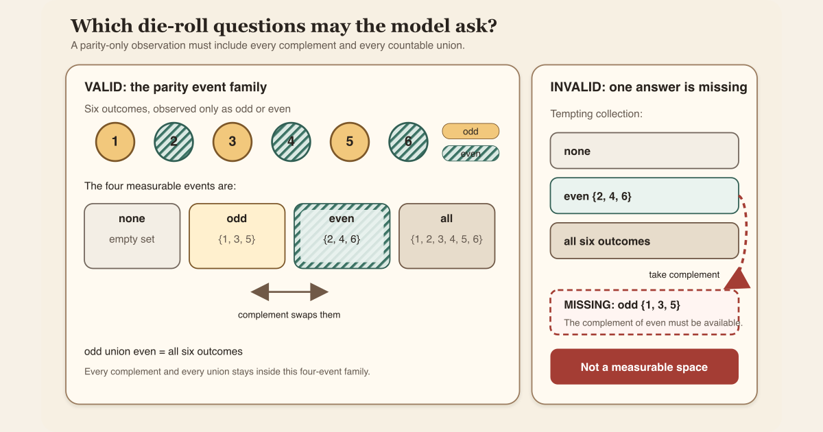
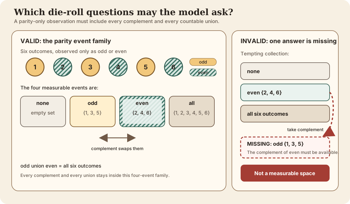
be the outcomes of one six-sided die roll. Imagine a sensor that reports only whether the result is odd or even. Define

The event family visible to that sensor is

This family is valid:

• the empty event \(\varnothing\) is present;
• taking a complement swaps \(O\) and \(E\), while it swaps \(\varnothing\) and \(\Omega\); and
• unions stay in the family, with \(O\cup E=\Omega\).

Even though a countable union may list infinitely many terms, every listed term is one of these four sets. If both \(O\) and \(E\) occur, the union is \(\Omega\); if only one occurs, the union is that one; and if every term is empty, the union is empty. Thus the countable-union rule also closes.

For a fair die, a probability rule on this coarse event family gives

It does not let the parity-only model ask for the probability of the singleton \(\{2\}\), because that exact-face question is not in \(\mathcal F\). A different measurable space on the same six outcomes could include every subset and therefore retain the complete die result.

The direct definition

Let \(\mathcal P(\Omega)\) denote the set of all subsets of \(\Omega\). A collection

is a sigma algebra when it satisfies three closure rules:

1. \(\varnothing\in\mathcal F\);

2. if \(A\in\mathcal F\), then its complement \(A^{\mathsf c}=\Omega\setminus A\) also belongs to \(\mathcal F\); and

3. if \(A_0,A_1,A_2,\ldots\) all belong to \(\mathcal F\), then

   \[ \bigcup_{n=0}^{\infty}A_n\in\mathcal F. \]

The whole space follows from the first two rules because \(\Omega=\varnothing^{\mathsf c}\). Countable intersections follow by taking complements and using De Morgan’s law. Thus the event family supports the logical operations not, or, and and without leaving the domain on which the measure theory is meant to operate.

The pair \((\Omega,\mathcal F)\) is a measurable space. No numerical measure has been chosen yet. A measurable space says which questions are admissible; a measure later assigns sizes to those questions.

A tempting collection that fails

Consider

It contains the empty event, the whole space, and the useful question “was the roll even?” It is nevertheless not a sigma algebra: the complement of \(E\) is \(O\), and \(O\notin\mathcal G\).

The failure has a plain-language interpretation. If a sensor can answer “even,” it can also answer “not even.” An information system closed under negation cannot keep the first event while discarding its complement.

Finiteness alone does not rescue an arbitrary event list. Every subset of a finite outcome space is perfectly well-defined, but only a collection obeying the closure rules is a measurable-space structure.

Why a function must be measurable

Let \((\Omega,\mathcal F)\) and \((Y,\mathcal G)\) be measurable spaces. A function

is measurable when every measurable target question pulls back to a measurable source question:

Here

is the preimage of \(B\). The arrow points backward from a question about reported values to the source outcomes that produce those values.

For the parity-only die, let

report parity, and let every subset of the two-value target be measurable. The preimages of the four target events are exactly \(\varnothing,O,E,\Omega\), so \(p\) is measurable.

By contrast, let \(r:\Omega\to\Omega\) report the exact face, give its target all subsets, but retain the parity-only structure on its source. Then

The exact-face readout is not measurable from that coarse source structure. Measurability therefore depends on both the function and the measurable structures placed on its domain and codomain.

The matrix case

A matrix is determined by its entries. The project gives a matrix space the entrywise measurable structure, so a matrix-valued map \(X\) is measurable exactly when every scalar coordinate map

is measurable. This turns one structured target into a family of ordinary scalar proof obligations.

For direct Hermitian assembly, each output entry is one of three forms: a real diagonal coordinate embedded in \(\mathbb C\), a strict-upper complex coordinate, or the complex conjugate of a reflected upper coordinate. The Hermitian coordinate space entry explains that assembly. The coordinatewise measurability criterion then checks each branch separately.

In Lean: a matrix map is measurable entry by entry

RandomMatrix.measurable_iff_entries X

The exact checked theorem is:

theorem measurable_iff_entries (X : RandomMatrix Ω ι κ 𝕜) :
    Measurable X ↔ ∀ i j, Measurable fun ω ↦ X ω i j := by
  rw [measurable_comap_iff]
  change Measurable (fun ω i j ↦ X ω i j) ↔ _
  simp only [measurable_pi_iff]

The first rewrite exposes the measurable structure pulled back from the function representation of matrices. The final theorem measurable_pi_iff says that a function-valued map is measurable exactly when every coordinate is measurable.

Check the parity closure rules locally

This small Std worksheet represents each die event as a sorted list. It checks all four complements and all sixteen pairwise unions in the parity family, then exposes the missing complement in the invalid family. Save it as /tmp/MeasurableSpaceScratch.lean on a normal Mac or Linux computer:

import Std

namespace MeasurableSpaceScratch

def faces : List Nat := [1, 2, 3, 4, 5, 6]
def odds : List Nat := [1, 3, 5]
def evens : List Nat := [2, 4, 6]

def parityFamily : List (List Nat) :=
  [[], odds, evens, faces]

def complement (event : List Nat) : List Nat :=
  faces.filter (fun face => !(event.contains face))

def union (left right : List Nat) : List Nat :=
  faces.filter (fun face => left.contains face || right.contains face)

def inParityFamily (event : List Nat) : Bool :=
  parityFamily.contains event

def complementChecks : List Bool :=
  parityFamily.map (fun event => inParityFamily (complement event))

def everyUnionStays : Bool :=
  parityFamily.all (fun left =>
    parityFamily.all (fun right => inParityFamily (union left right)))

def invalidFamily : List (List Nat) :=
  [[], evens, faces]

#eval complementChecks
#eval everyUnionStays
#eval complement evens
#eval invalidFamily.contains (complement evens)

example : complementChecks = [true, true, true, true] := by decide
example : everyUnionStays = true := by decide
example : complement evens = odds := by decide
example : invalidFamily.contains (complement evens) = false := by decide

end MeasurableSpaceScratch

Type these commands exactly:

source "$HOME/.elan/env"
elan run leanprover/lean4:v4.32.0 lean /tmp/MeasurableSpaceScratch.lean

This exact standalone worksheet was executed successfully with Lean 4.32.0. It printed:

[true, true, true, true]
true
[1, 3, 5]
false

The first two lines verify the finite closure ledger. The final two say that the complement of the even faces is the odd set and that the tempting three-event family omits it. This is a finite model of the closure rules, not a replacement for Mathlib’s general countable-union structure.

Full project check

The next worksheet is a full project check. It uses the repository’s pinned Lean and Mathlib dependencies and may require substantial disk space and memory:

import NonlinearDynamics.Random.RandomMatrices.Basic

open NonlinearDynamics.Random

#check MeasurableSpace
#check MeasurableSet
#check Measurable
#check RandomMatrix.measurable_iff_entries
#check RandomMatrix.measurable_entry

example {Ω ι κ 𝕜 : Type*}
    [MeasurableSpace Ω] [MeasurableSpace 𝕜]
    (X : RandomMatrix Ω ι κ 𝕜)
    (hX : Measurable X) (i : ι) (j : κ) :
    Measurable (fun ω ↦ X ω i j) :=
  RandomMatrix.measurable_entry hX i j

The three general #check commands ask Lean for the core measurable-space interfaces. The two project commands ask for the exact matrix criterion and its one-entry consequence. The final pedagogical example applies the same checked project theorem to extract one measurable entry from a measurable matrix-valued function.

cd formalization
lake env lean -DwarningAsError=true NonlinearDynamics/Random/RandomMatrices/Basic.lean

Boundaries and common misconceptions

• A measurable space is not a measure. It chooses the admissible events; it does not assign any event a number.
• Measurable does not mean likely. A measurable event can have probability zero, one, or anything between once a probability measure is chosen.
• Measurable does not mean integrable. Measurability makes inverse-image questions legitimate. Integrability separately controls the size of a function.
• Measurable does not mean continuous. Every continuous map between the usual real Borel spaces is measurable, but many measurable maps are discontinuous.
• Finite does not mean every proposed family works. The failed \(\mathcal G\) example is finite but not complement-closed.
• The same bare function can change status. Coarsening its target or refining its source can make measurability easier; refining its target or coarsening its source can make it harder.
• Matrix measurability adds no distributional assumptions. It does not imply independent entries, Gaussian entries, finite moments, Hermiticity, or a particular probability distribution .

Where to continue

The random matrix entry separates one matrix-valued sample map from a realized matrix and from its law. The probability distribution entry then shows why measurability is required before probability can be pushed through a function. The almost everywhere entry explains how a chosen measure later permits exceptional sets of measure zero.

For the first finite product application, the finite random-matrix product entry proves that only the factors in the selected prefix need measurable coordinate maps before the product law can be formed.

References

Mathlib contributors. Measurable spaces and measurable functions, Mathlib 4 documentation. The pinned source defines MeasurableSpace, MeasurableSet, and Measurable, including the preimage-based implementation used by the project.

Nonlinear Dynamics in Lean contributors. Random-matrix foundation module, the checked project source for the entrywise matrix measurable space, measurable_iff_entries, and the coordinatewise closure theorems.