Measure

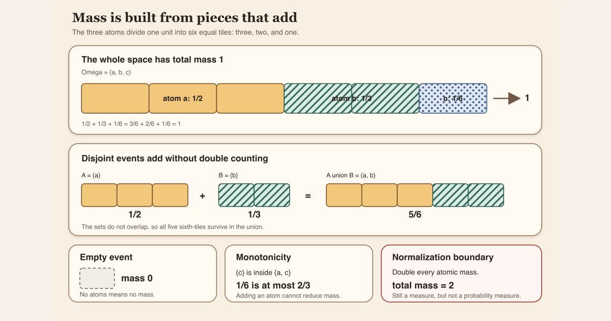
A measure assigns a nonnegative mass to each measurable event. Here an event is a subset of the possible outcomes, and “measurable” means that the subset belongs to the chosen measurable space . A measure can describe length, area, volume, counting, physical mass, or probability. Probability is the special case in which the whole outcome space has mass \(1\).

The finite example below exhibits the central rule: disjoint pieces can be weighed separately and their masses added.

Start with three atoms

Let the outcome space be

\[ \Omega=\{a,b,c\}. \]

An atom in this example is one indivisible outcome. Give the three atoms the exact masses

Atom	Mass	Mass in sixths
\(a\)	\(1/2\)	\(3/6\)
\(b\)	\(1/3\)	\(2/6\)
\(c\)	\(1/6\)	\(1/6\)

Every subset of this finite space will be measurable. For an event \(S\subseteq\Omega\), define

\[ \mu(S)=\sum_{x\in S}w_x, \qquad w_a=\frac12, \quad w_b=\frac13, \quad w_c=\frac16. \]

The symbol \(\mu\), pronounced “mu,” names the measure. The notation \(\mu(S)\) means “evaluate the measure at the set \(S\).” It is a number, not another set.

This one definition already gives several computations:

\[ \mu(\varnothing)=0 \]

because there are no atomic masses to add, while

\[ \mu(\{a,c\})=\frac12+\frac16=\frac23. \]

Take \(A=\{a\}\) and \(B=\{b\}\). They are disjoint, meaning \(A\cap B=\varnothing\). Therefore no atom is counted twice, and

\[ \mu(A\cup B) =\mu(\{a,b\}) =\frac12+\frac13 =\frac56 =\mu(A)+\mu(B). \]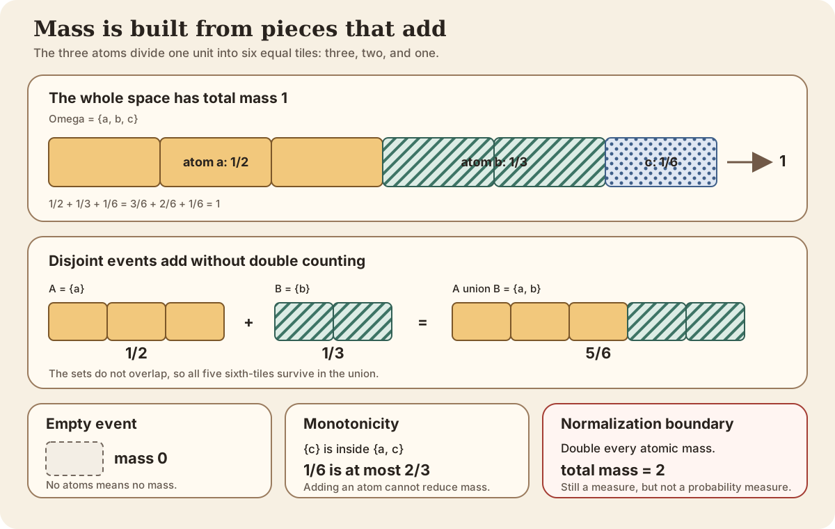

Six equal mass tiles are divided among atoms a, b, and c in groups of three, two, and one. The three tiles of event A and two tiles of disjoint event B join to form five tiles for their union. Separate cards show empty mass zero, monotonicity, and a doubled measure with total mass two. — FigureFinding: exact mass arithmetic is visible as tile arithmetic. Atom \(a\) owns \(3/6=1/2\), atom \(b\) owns \(2/6=1/3\), and atom \(c\) owns \(1/6\), so the whole space has mass \(1\). The disjoint events \(A=\{a\}\) and \(B=\{b\}\) contribute three and two tiles, hence \(\mu(A\cup B)=5/6=1/2+1/3\). The empty event owns no tiles. Since \(\{c\}\subseteq\{a,c\}\), its mass \(1/6\) is at most \(2/3\). Doubling every atomic mass produces a valid measure of total mass \(2\), but not a probability measure.

The direct definition

Let \((\Omega,\mathcal F)\) be a measurable space. A measure is a function

\[ \mu:\mathcal F\longrightarrow[0,\infty] \]

with two defining properties.

The empty event has no mass:
\[ \mu(\varnothing)=0. \]
If \(A_0,A_1,A_2,\ldots\) are measurable and pairwise disjoint, then
\[ \mu\!\left(\bigcup_{n=0}^{\infty}A_n\right) =\sum_{n=0}^{\infty}\mu(A_n). \]

Pairwise disjoint means that every two different events in the list have empty intersection. The target \([0,\infty]\) is the extended nonnegative real line: it contains every ordinary nonnegative real number and also the value \(\infty\). Allowing infinite mass lets one measure an unbounded line by length, for example.

The second rule is called countable additivity. The familiar two-set rule

\[ A\cap B=\varnothing \quad\Longrightarrow\quad \mu(A\cup B)=\mu(A)+\mu(B) \]

is its finite shadow. If \(A\) and \(B\) overlap, the right side counts the intersection twice, so this equality is no longer the correct general rule.

Another consequence is monotonicity:

\[ A\subseteq B \quad\Longrightarrow\quad \mu(A)\leq\mu(B). \]

In the three-atom example, \(\{c\}\subseteq\{a,c\}\), and indeed

\[ \mu(\{c\})=\frac16\leq\frac23=\mu(\{a,c\}). \]

Mathlib represents a measure as a function that can be evaluated on every set, not only on a set accompanied by a measurability proof. Internally, its outer-measure construction supplies that total function. The exact additive equalities used in ordinary measure theory still ask for the relevant measurability hypotheses. This implementation detail should not be mistaken for permission to ignore the measurable space.

Why this example is also probability

The total mass in the example is

\[ \mu(\Omega) =\frac12+\frac13+\frac16 =\frac36+\frac26+\frac16 =1. \]

A measure with total mass \(1\) is a probability measure. Thus this particular \(\mu\) can assign probabilities to events. A random variable then transports that source probability measure to a probability law on its value space.

Normalization is extra structure, not part of the definition of a measure. For a sharp counterexample, double every atomic mass and write

\[ \nu(S)=2\mu(S). \]

The rule \(\nu\) is still nonnegative, gives the empty set mass zero, and is countably additive. But

\[ \nu(\Omega)=2, \]

so \(\nu\) is a measure and is not a probability measure.

A measure is not a density

A measure directly answers a set question: “what is the mass of \(A\)?” A density answers a different, relative question: “how is that mass spread with respect to some already chosen reference measure \(\lambda\)?” When such a density \(\rho\) exists, the relationship is

\[ \mu(A)=\int_A \rho\,d\lambda. \]

The density depends on the reference measure. It is not the measure itself. Moreover, a density need not exist for a particular reference. For example, a point mass at \(0\) gives the singleton \(\{0\}\) positive mass. Ordinary length measure gives that singleton mass zero, so no ordinary function density with respect to length can reproduce the point mass.

On the three-point space, counting measure is a convenient reference: it gives each atom mass \(1\), and the density values are \(\rho(a)=1/2\), \(\rho(b)=1/3\), and \(\rho(c)=1/6\). That is a feature of the chosen finite reference, not a universal identification of measures with densities.

In Lean: disjoint events add

One idea, three languages Read across, then read the syntax map

A human says

If two events do not overlap and the second event is measurable, the mass of their union is the sum of their masses.

On paper

\((A\cap B=\varnothing)\land(B\in\mathcal F)\Longrightarrow\mu(A\cup B)=\mu(A)+\mu(B).\)

In Lean

measure_union hAB hB

Syntax map

μ A is ordinary function application in Lean. A human types the measure name, a space, and the set name; paper usually adds parentheses and writes \(\mu(A)\).
A ∪ B is the set union \(A\cup B\).
hAB : Disjoint A B is a named proof that \(A\) and \(B\) do not overlap. For sets, this says \(A\cap B=\varnothing\).
hB : MeasurableSet B is a named proof that \(B\) belongs to the measurable event family.
measure_union is Mathlib’s checked theorem. Its interface asks for measurability of the second set; its implementation can evaluate the first set through the outer-measure representation. In standard event arithmetic, readers will usually know both sets are measurable.
A value such as μ A has type ℝ≥0∞, Mathlib’s notation for the extended nonnegative reals \([0,\infty]\).

Small standalone tutorial: add the three atomic masses

To keep the finite arithmetic exact without importing a rational-number or measure library, record every mass in sixths. The values \(3\), \(2\), and \(1\) below mean \(3/6\), \(2/6\), and \(1/6\). An event is represented by a duplicate-free list of its atoms. Create /tmp/ThreeAtomMeasure.lean with these contents:

import Std

namespace ThreeAtomMeasure

inductive Atom
  | a
  | b
  | c
  deriving DecidableEq, Repr

def weightSixths : Atom → Nat
  | .a => 3
  | .b => 2
  | .c => 1

def massSixths (event : List Atom) : Nat :=
  event.foldl (fun total atom => total + weightSixths atom) 0

#eval [
  massSixths [],
  massSixths [.a],
  massSixths [.b],
  massSixths [.a, .b],
  massSixths [.a, .c],
  massSixths [.a, .b, .c]
]
#eval 2 * massSixths [.a, .b, .c]

example :
    massSixths [.a, .b] = massSixths [.a] + massSixths [.b] := by
  decide

example : massSixths [.a, .c] = 4 := by decide
example : massSixths [.a, .b, .c] = 6 := by decide
example : 2 * massSixths [.a, .b, .c] = 12 := by decide

end ThreeAtomMeasure

From any directory on a normal macOS or Linux machine with the pinned compiler, type exactly:

source "$HOME/.elan/env"
elan run leanprover/lean4:v4.32.0 lean /tmp/ThreeAtomMeasure.lean

This exact worksheet was executed successfully with Lean 4.32.0 while repairing this page. It printed:

[0, 3, 2, 5, 4, 6]
12

The first output is the sixths ledger for the empty event, \(A\), \(B\), \(A\cup B\), \(\{a,c\}\), and the whole space. The second is the doubled measure’s total mass in sixths, namely \(12/6=2\). The duplicate-free-list convention matters: a repeated atom would incorrectly count the same event member twice. This is a bounded Std tutorial, not Mathlib’s general countably additive measure construction.

Exact project and Mathlib interface

Here is a complete worksheet a human can type into a scratch .lean file on a clone with the repository’s pinned dependencies installed:

import NonlinearDynamics.Random.RandomMatrices.Laws

open Set MeasureTheory
open NonlinearDynamics.Random

#check Measure
#check measure_empty
#check measure_mono
#check measure_union
#check RandomMatrix.law
#check RandomMatrix.law_apply

variable {Ω : Type*} [MeasurableSpace Ω]
variable (μ : Measure Ω) (A B : Set Ω)

#check μ A

example (hAB : Disjoint A B) (hB : MeasurableSet B) :
    μ (A ∪ B) = μ A + μ B := by
  exact measure_union hAB hB

Read the typed expression μ A as the paper expression \(\mu(A)\). The line #check μ A asks Lean to infer and display its type. The example supplies the two named hypotheses to measure_union, and Lean’s kernel checks the resulting proof of the displayed disjoint-additivity statement.

The imported project module is not arbitrary. It defines the law of a random matrix from an explicit source μ : Measure Ω. Its theorem RandomMatrix.law_apply evaluates the transported measure by evaluating that source measure on a preimage:

\[ \mathcal L_\mu(X)(s)=\mu(X^{-1}(s)). \]

In Lean, the right side is typed μ (X ⁻¹’ s). The symbols ⁻¹’ denote a set preimage, not an inverse function.

Try it in the repository NonlinearDynamics/Random/RandomMatrices/Laws.lean

The authoritative project source is formalization/NonlinearDynamics/Random/RandomMatrices/Laws.lean. It accepts an arbitrary source Measure Ω, proves the measurable-set evaluation theorem RandomMatrix.law_apply, and separately proves that a probability source produces a probability law. #check in the worksheet above only asks Lean to elaborate a declaration or expression; the final example is the line that checks the stated theorem in the reader’s scratch file. The full-project command checks the full module with the repository’s pinned dependencies installed.

Full project check, from the repository root

cd formalization
lake env lean -DwarningAsError=true NonlinearDynamics/Random/RandomMatrices/Laws.lean

Resource note: this exact file uses the repository's pinned Lean and Mathlib dependencies. Initial project setup can require substantial disk space and build time. For a lightweight first step on macOS or Linux, use the page's standalone Lean-core or Std tutorial.

Distinctions and failure modes

Tempting shortcut	What is wrong	Correct repair
“The event and its measure are the same thing”	\(A\) is a set, while \(\mu(A)\) is an extended nonnegative number	Keep the input set and output mass separate
“A measurable space already assigns probabilities”	It specifies admissible events but contains no numerical weights	Choose a measure after choosing the measurable space
“Every measure is a probability measure”	A measure may have total mass \(2\), \(37\), or \(\infty\)	Check the extra normalization \(\mu(\Omega)=1\)
“A measure is a density”	A density is relative to another measure and may not exist for the chosen reference	State the reference measure and prove a density representation
“Mass zero means the event is empty”	A nonempty set can have measure zero	Distinguish emptiness from a null set
“Masses always add across a union”	Overlap would be counted twice	Require disjointness, or subtract the intersection when a finite formula permits it
“A smaller event can have more mass”	Nonnegativity and additivity force monotonicity	From \(A\subseteq B\), conclude \(\mu(A)\leq\mu(B)\)

Where to continue

Read measurable space for the event family on which measure arithmetic is justified. Read null set for nonempty events of mass zero, and almost everywhere for statements that may fail only on such an event. Then read pushforward measure for transporting mass through a measurable function and probability law for the normalized law of a random object.

References

Mathlib contributors. Measures, Mathlib 4 documentation. This official implementation reference contains the evaluation interface and theorems measure_empty, measure_mono, and measure_union used in the worksheet.

Mathlib contributors. Probability measure typeclass, Mathlib 4 documentation. This official source records the additional whole-space normalization used to distinguish probability measures from general measures.

Olav Kallenberg. Foundations of Modern Probability, third edition, Springer, 2021. This is a standard reference for measures, probability spaces, random elements, and their distributions.