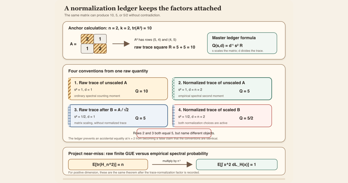
A normalization convention is an explicit agreement about scale. It says which object is being scaled, by what factor, whether a trace or measure is divided by dimension, what a variance parameter means, and how boundary cases are handled.
These choices are not cosmetic. They change exact answers. Two authors can start from the same matrix and correctly report \(10\), \(5\), or \(5/2\) because they asked three different normalized questions.
The safest practice is to keep a normalization ledger beside every theorem: a short table whose factors accompany the notation.
Start with one matrix and one raw quantity
Take the \(2\times2\) Hermitian matrix
\[ A= \begin{bmatrix} 2&1\\ 1&2 \end{bmatrix}. \]Its square is
\[ A^2= \begin{bmatrix} 5&4\\ 4&5 \end{bmatrix}, \]so the raw second trace power is
\[ R=\operatorname{tr}(A^2)=5+5=10. \]This calculation is the fixed anchor. Every quantity below is obtained by attaching explicit scale factors to this same \(R\).
One formula contains the common conventions
Suppose the matrix is first scaled by a scalar \(s\), and the trace is then divided by a positive divisor \(d\). At power \(k\), define
\[ Q_{s,d,k}(A) =\frac1d\operatorname{tr}\bigl((sA)^k\bigr). \]Scalar multiplication commutes with matrix powers, so
\[ Q_{s,d,k}(A) =d^{-1}s^k\operatorname{tr}(A^k). \]The matrix scale contributes the \(k\)-th power \(s^k\). The trace normalization contributes a separate factor \(d^{-1}\). Combining them in one formula prevents one factor from impersonating the other.
For the worked example, \(n=2\), \(k=2\), and \(R=10\):
| Convention | Matrix scale \(s\) | Trace divisor \(d\) | Calculation | Value |
|---|---|---|---|---|
| Raw trace of \(A^2\) | \(1\) | \(1\) | \(1\cdot1\cdot10\) | \(10\) |
| Normalized trace of \(A^2\) | \(1\) | \(n=2\) | \(1\cdot1\cdot10/2\) | \(5\) |
| Raw trace of \((A/\sqrt2)^2\) | \(1/\sqrt2\) | \(1\) | \((1/2)\cdot10\) | \(5\) |
| Normalized trace of \((A/\sqrt2)^2\) | \(1/\sqrt2\) | \(n=2\) | \((1/2)\cdot10/2\) | \(5/2\) |
The near-miss: equal numbers, unequal conventions
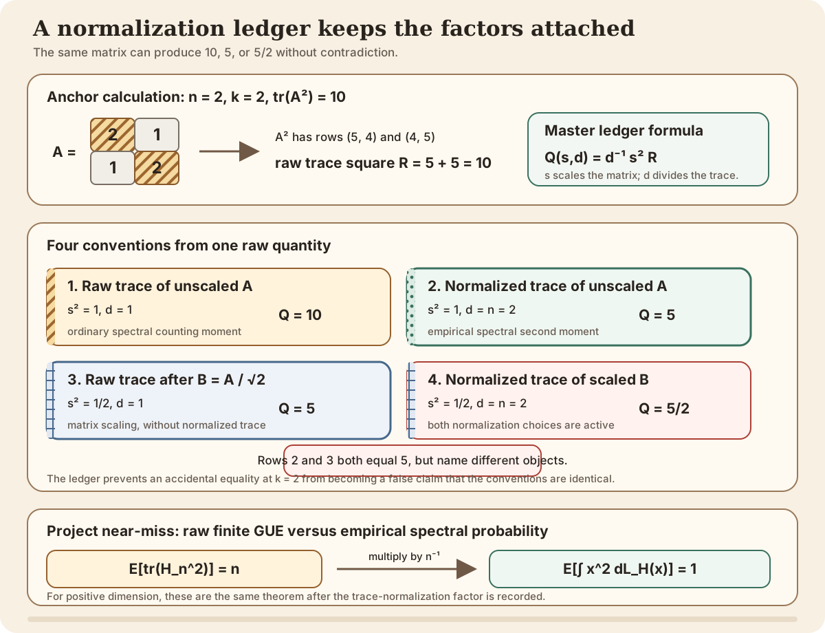
The second and third rows both equal \(5\):
\[ \frac12\operatorname{tr}(A^2) =\operatorname{tr}\!\left(\left(\frac{A}{\sqrt2}\right)^2\right). \]It would be a mistake to conclude that normalized trace and matrix scaling are the same operation. They happen to contribute the same factor at \(n=2\) and \(k=2\):
\[ n^{-1}=n^{-k/2}=\frac12. \]Change the power to \(k=1\). The normalized trace of the unscaled matrix is
\[ \frac12\operatorname{tr}(A)=\frac12\cdot4=2, \]while the raw trace of the scaled matrix is
\[ \operatorname{tr}\!\left(\frac{A}{\sqrt2}\right) =\frac4{\sqrt2} =2\sqrt2. \]The accidental equality disappears. A normalization comparison must match the formula, not merely one numerical test case.
The general dimension factors
For an \(n\times n\) matrix \(A\):
| Quantity | Exact factor multiplying \(\operatorname{tr}(A^k)\) |
|---|---|
| Ordinary trace power | \(1\) |
| Normalized trace power | \(n^{-1}\) |
| Ordinary trace after \(A\mapsto A/\sqrt n\) | \(n^{-k/2}\) |
| Normalized trace after \(A\mapsto A/\sqrt n\) | \(n^{-1-k/2}\) |
The normalized trace is the \(k\)-th moment of the empirical spectral probability measure :
\[ L_A=\frac1n\sum_{i=1}^n\delta_{\lambda_i}, \qquad \int x^k\,dL_A(x)=\frac1n\operatorname{tr}(A^k). \]The ordinary trace power is instead the moment of the unnormalized spectral counting measure \(\sum_i\delta_{\lambda_i}\), whose total mass is \(n\). Measure normalization and matrix scaling are again separate ledger rows.
A practical normalization ledger
Before comparing a paper, a plot, and a Lean theorem, record at least:
| Ledger field | Question to answer | Worked example |
|---|---|---|
| Base object | Which matrix or random matrix is named? | \(A\) |
| Dimension | What is \(n\), including its zero policy? | \(n=2\) |
| Matrix scale | Is the object \(A\), \(A/\sqrt n\), or something else? | \(s=1\) or \(1/\sqrt2\) |
| Power | Which exponent is used? | \(k=2\) |
| Trace convention | Ordinary trace or \(n^{-1}\operatorname{tr}\)? | \(d=1\) or \(2\) |
| Spectral measure | Counting mass \(n\) or empirical mass \(1\)? | \(N_A\) or \(L_A\) |
| Probability layer | Sample value, expectation, or law? | deterministic sample value |
| Entry variance | Variance or standard deviation, and before or after scaling? | not applicable here |
| Scalar type | In which number system is division interpreted? | real or complex |
| Boundary rule | What happens at \(n=0\)? | must be stated separately |
A ledger prevents three common false comparisons:
- comparing a raw trace theorem with a normalized-trace theorem;
- comparing an unscaled ensemble with a Wigner-scaled ensemble; and
- comparing a deterministic sample statistic with its expectation.
When translating a paper into Lean, the ledger also identifies exactly where each factor appears in the term. If a reciprocal dimension is not visible in the statement or in a named definition, it has not been supplied by prose.
The project’s Wigner ledger
The finite GUE construction uses a Wigner normalization with an explicit zero-dimensional branch. For positive dimension \(n\):
- each real diagonal coordinate has variance \(1/n\);
- the real and imaginary parts of each strict-upper coordinate each have variance \(1/(2n)\);
- the assembled matrix law is a probability measure;
- the expected ordinary second trace power is \(n\); and
- the expected second moment of the empirical spectral probability measure is \(1\).
The last two statements are not contradictory:
\[ \mathbb E[\operatorname{tr}(H_n^2)]=n, \]while
\[ \mathbb E\!\left[\int x^2\,dL_{H_n}(x)\right] =\mathbb E\!\left[\frac1n\operatorname{tr}(H_n^2)\right] =1 \]for positive \(n\). The normalization ledger turns the apparent disagreement \(n\) versus \(1\) into the exact identity \(n^{-1}n=1\).
Dimension zero cannot be handled by an informal instruction to divide by \(n\). The project defines its variance scale and empirical spectral measure separately at zero. This makes the boundary total and testable rather than leaving a hidden division-by-zero obligation.
Variance conventions use the same discipline
Normalization problems are not limited to traces. For independent centered real variables \(U\) and \(V\) of variance \(1\), compare
\[ Z_1=\frac{U+iV}{\sqrt2}, \qquad Z_2=U+iV. \]Then
\[ \mathbb E|Z_1|^2=1, \qquad \mathbb E|Z_2|^2=2. \]Both are valid complex Gaussian conventions. The first has real and imaginary component variance \(1/2\); the second has component variance \(1\). Saying “unit variance” without specifying component variance or total squared magnitude leaves the ledger incomplete.
The same square law appears whenever a scalar random variable is rescaled:
\[ \operatorname{Var}(cX)=c^2\operatorname{Var}(X). \]Read variance and Gaussian distribution for those probability conventions. The matrix ledger adds dimension, trace, and spectral measure choices on top.
In Lean: the reciprocal dimension is visible
The project theorem for a deterministic Hermitian matrix states that its second empirical spectral moment is the reciprocal-dimension normalized trace square.
NonlinearDynamics.Random.RandomMatrix.empiricalSpectralMoment_two HH : HermitianEuclidean nis the bundled \(n\times n\) Hermitian matrix.empiricalSpectralMoment 2 His the integral of(x : ℂ) ^ 2against the empirical spectral measure.- The theorem’s right side begins
(((n : ℕ) : ℝ)⁻¹ : ℂ). Lean first regardsnas a natural number, casts it to a real number, takes its reciprocal, and then casts that coefficient to a complex number. - The explicit coefficient is multiplied by
Matrix.trace ((hermitianToMatrix H) ^ 2). hermitianToMatrix Hexposes the ambient complex matrix.^ 2is matrix squaring;Matrix.traceis the ordinary, unnormalized trace.- A human types the fully qualified name
NonlinearDynamics.Random.RandomMatrix.empiricalSpectralMoment_two Hwhen a proof of this complete equality is needed. Lean does not infer the intended normalization from the phrase “spectral moment.”
The exact checked theorem is:
theorem empiricalSpectralMoment_two {n : ℕ} (H : HermitianEuclidean n) :
    empiricalSpectralMoment 2 H =
      (((n : ℕ) : ℝ)⁻¹ : ℂ) * Matrix.trace ((hermitianToMatrix H) ^ 2) := by
  rw [empiricalSpectralMoment, empiricalSpectralMeasure,
    integral_smul_measure, ENNReal.toReal_inv]
  rw [integral_sq_complex_ofReal_spectralCountingMeasure]
  norm_cast
The project also records the Wigner entry scale without overloading the symbol \(n^{-1}\):
noncomputable def varianceScale : ℕ → ℝ≥0
  | 0 => 0
  | n + 1 => (((n + 1 : ℕ) : ℝ≥0))⁻¹

noncomputable def diagonalVariance (n : ℕ) : ℝ≥0 := varianceScale n

noncomputable def upperCartesianVariance (n : ℕ) : ℝ≥0 :=
  varianceScale n / 2
Thus the diagonal variance and each upper Cartesian component variance have different names and formulas. The positive-dimensional reciprocal is explicit, and the zero branch is not hidden behind a field convention.
Finally, the two ensemble outputs expose both trace conventions. The
declaration GUE.integral_tracePower_two n concludes that the raw
second trace-power integral equals (n : ℂ). The normalized
positive-dimensional declaration is short enough to quote with its complete
checked proof:
@[simp] theorem integral_empiricalSpectralMoment_two_succ (n : ℕ) :
    ∫ H, empiricalSpectralMoment 2 H ∂intrinsicLaw (n + 1) = 1 := by
  rw [integral_empiricalSpectralMoment_two]
  norm_cast
  exact inv_mul_cancel₀ (by positivity)
The project-source worksheet below asks Lean for the exact type of both declarations. The project build, not a prose paraphrase, is the authority for their complete proofs.
Standalone tutorial: exact ledger
Standalone tutorial. This worksheet imports only
Std and uses exact rational arithmetic. It does not import
Mathlib or the project.
Save the following as NormalizationLedgerScratch.lean:
import Std

structure TraceLedger where
  dimension : Rat
  matrixScaleSquared : Rat
  traceDivisor : Rat
deriving Repr

def applySecondPowerLedger
    (ledger : TraceLedger) (rawTraceSquare : Rat) : Rat :=
  ledger.matrixScaleSquared * rawTraceSquare / ledger.traceDivisor

def rawUnscaled : TraceLedger :=
  { dimension := 2, matrixScaleSquared := 1, traceDivisor := 1 }

def normalizedUnscaled : TraceLedger :=
  { dimension := 2, matrixScaleSquared := 1, traceDivisor := 2 }

def rawScaled : TraceLedger :=
  { dimension := 2, matrixScaleSquared := (1 : Rat) / 2,
    traceDivisor := 1 }

def normalizedScaled : TraceLedger :=
  { dimension := 2, matrixScaleSquared := (1 : Rat) / 2,
    traceDivisor := 2 }

#eval applySecondPowerLedger rawUnscaled 10
#eval applySecondPowerLedger normalizedUnscaled 10
#eval applySecondPowerLedger rawScaled 10
#eval applySecondPowerLedger normalizedScaled 10
Run it with:
elan run leanprover/lean4:v4.32.0 lean NormalizationLedgerScratch.lean
The four exact outputs should be \(10\), \(5\), \(5\), and \(5/2\). The
dimension field is deliberately recorded even though the tiny
function uses the already-selected traceDivisor. That redundancy
lets a reviewer check whether the divisor really matches the stated dimension.
Project-source workflow
Full project check. This uses the repository’s pinned Lean and Mathlib
dependencies and may require substantial disk space and memory.
The main authoritative source
for the normalized spectral statement is
formalization/NonlinearDynamics/Random/RandomMatrices/GaussianUnitaryEnsembleSpectrum.lean.
Its upstream scale and raw-moment declarations live in
GaussianUnitaryEnsemble.lean
and
GaussianUnitaryEnsembleMoments.lean.
A human can type:
import NonlinearDynamics.Random.RandomMatrices.GaussianUnitaryEnsembleSpectrum

#check NonlinearDynamics.Random.GUE.varianceScale
#check NonlinearDynamics.Random.GUE.varianceScale_zero
#check NonlinearDynamics.Random.GUE.varianceScale_succ
#check NonlinearDynamics.Random.RandomMatrix.empiricalSpectralMoment
#check NonlinearDynamics.Random.RandomMatrix.empiricalSpectralMoment_two
#check NonlinearDynamics.Random.GUE.integral_tracePower_two
#check NonlinearDynamics.Random.GUE.integral_empiricalSpectralMoment_two_succ
Each #check displays the exact declaration type from the pinned
source. It does not compute the local matrix example or compare conventions on
the reader’s behalf. The full-project command below checks the full spectrum
module and its imported dependencies.
cd formalization
lake env lean -DwarningAsError=true NonlinearDynamics/Random/RandomMatrices/GaussianUnitaryEnsembleSpectrum.lean
Resource note: this exact file uses the repository's
pinned Lean and Mathlib dependencies. Initial project setup can require
substantial disk space and build time. For a lightweight first step on
macOS or Linux, use the page's standalone Lean-core or Std
tutorial.
Boundaries and failure modes
| Tempting shortcut | What is wrong | Correct repair |
|---|---|---|
| “Normalized matrix means normalized trace” | Scaling entries and dividing the final trace contribute different powers | Record matrix scale \(s\) and trace divisor \(d\) separately |
| “Both formulas gave five, so they use the same convention” | Equality at one dimension and power may be accidental | Compare the symbolic factors \(d^{-1}s^k\) |
| “Second moment means one universal quantity” | Counting and empirical spectral measures have different total mass | State the measure and its mass |
| “Variance one is unambiguous” | It may mean component variance, total complex variance, or standard deviation | Name the parameter and its units |
| “Expectation and sample value can be compared directly” | One averages over a law and the other evaluates one realization | Record the probability layer |
| “Division by dimension works at zero” | The informal reciprocal has no ordinary positive-dimensional meaning there | Publish an explicit zero-dimensional policy |
| “Lean will supply the convention from context” | Coercions and inverses are type-correct under many possible conventions | Keep the factor visible in a definition or theorem |
| “Changing scale preserves every theorem verbatim” | \(k\)-th moments acquire the \(k\)-th power of the scale | Transport the theorem with the exact exponent |
Where to continue
Read trace power for the matrix and spectral calculation behind the worked example. Read empirical spectral measure for the mass-one spectral normalization and finite matrix trace moment for the expectation layer. The Gaussian unitary ensemble entry records the project’s complete entrywise Wigner ledger.
Finite GUE from Independent Gaussian Coordinates builds the normalized law. First Exact Finite Gaussian Unitary Ensemble Trace Moments derives the raw \(n\)-valued second trace moment. Finite GUE Empirical Spectral Laws and Normalized Moments then applies reciprocal-dimension normalization to obtain the positive-size value \(1\).
References
Mathlib contributors. Gaussian distributions over the reals, Mathlib 4 documentation. This official API reference fixes the real Gaussian variance parameter used by the project’s entrywise law.
Terence Tao. Topics in Random Matrix Theory, Graduate Studies in Mathematics 132, American Mathematical Society, 2012. This reference discusses Wigner scaling, normalized traces, empirical spectral measures, and the moment method.
Greg W. Anderson, Alice Guionnet, and Ofer Zeitouni. An Introduction to Random Matrices, Cambridge University Press, 2010. This is a standard source for finite random-matrix normalization and asymptotic spectral conventions.
Nonlinear Dynamics in Lean contributors. GaussianUnitaryEnsembleSpectrum.lean, the checked project source connecting empirical spectral moments to normalized trace powers.