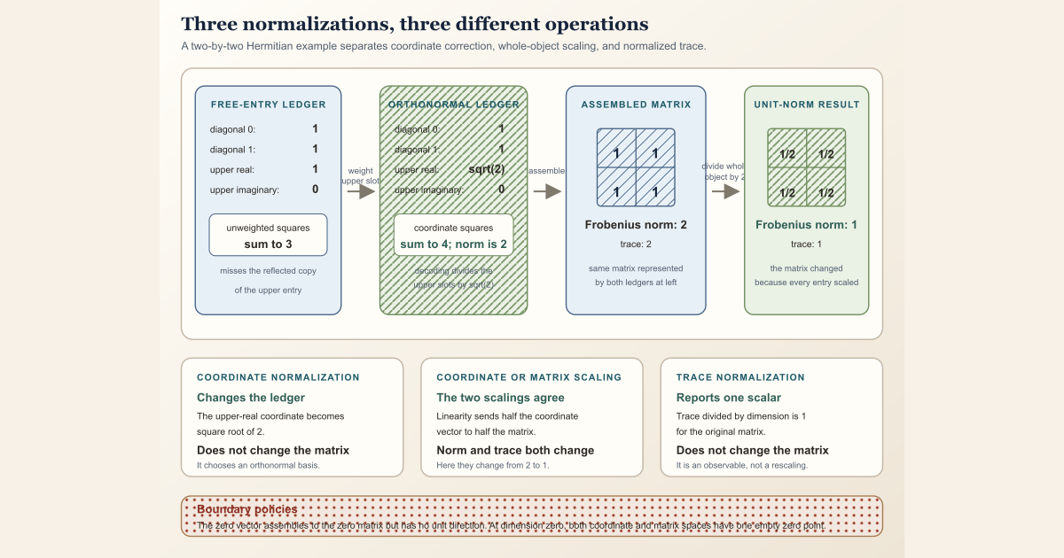
Normalized Hermitian coordinates are real coordinates for a finite Hermitian matrix chosen to be orthonormal for the Frobenius inner product. Diagonal entries are stored as they are. The real and imaginary parts of every freely chosen strict-upper entry are multiplied by \(\sqrt{2}\).
That factor has one job: it compensates for the conjugate copy below the diagonal. It makes ordinary Euclidean length in the coordinate ledger equal to Frobenius length of the assembled matrix.
Start with one exact two-by-two matrix
Consider
\[ H= \begin{pmatrix} 1&1\\ 1&1 \end{pmatrix}. \]This matrix is Hermitian: its diagonal entries are real, and its lower-left entry is the complex conjugate of its upper-right entry. A human can record its freely chosen data as
\[ q=(d_0,d_1,r,s)=(1,1,1,0), \]where \(r+is=1+0i\) is the upper-right entry. The lower-left entry is not a fifth independent choice. Hermitian symmetry determines it.
If we square only those four displayed numbers, we get
\[ \lVert q\rVert_{\mathrm{unweighted}}^2 =1^2+1^2+1^2+0^2 =3. \]But the Frobenius norm includes every matrix position:
\[ \lVert H\rVert_F^2 =|1|^2+|1|^2+|1|^2+|1|^2 =4. \]The raw free-entry ledger misses the second copy of the off-diagonal entry. To repair it, store
\[ x=(d_0,d_1,b,c) =(d_0,d_1,\sqrt{2}\,r,\sqrt{2}\,s) =(1,1,\sqrt{2},0). \]Now ordinary Euclidean arithmetic gives the right answer:
\[ \lVert x\rVert_2^2 =1^2+1^2+(\sqrt{2})^2+0^2 =4, \qquad \lVert x\rVert_2=2=\lVert H\rVert_F. \]Decoding divides the two normalized upper coordinates by \(\sqrt{2}\):
\[ D_2(x)= \begin{pmatrix} d_0 & (b+ic)/\sqrt{2}\\ (b-ic)/\sqrt{2} & d_1 \end{pmatrix} {} = \begin{pmatrix} 1&1\\ 1&1 \end{pmatrix} =H. \]The ledger changed from \(q\) to \(x\), but the represented matrix did not.
Unit length is a separate operation
Because \(x\ne0\) and \(\lVert x\rVert_2=2\), we may separately form the unit vector
\[ \widehat x =\frac{x}{\lVert x\rVert_2} =\left(\frac12,\frac12,\frac1{\sqrt{2}},0\right). \]Assembly is linear, so dividing the whole coordinate vector by two divides the whole matrix by two:
\[ D_2(\widehat x) =\frac12D_2(x) =\frac12H {} = \begin{pmatrix} 1/2&1/2\\ 1/2&1/2 \end{pmatrix}. \]This new matrix has Frobenius norm one. Unlike the earlier coordinate correction, this step really changes the matrix.
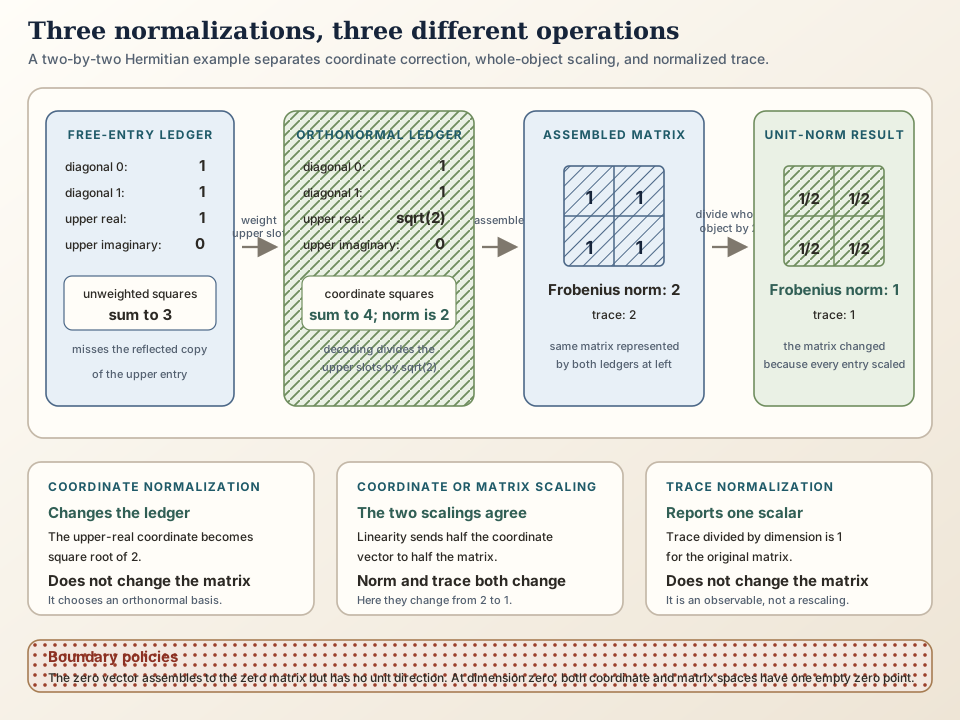
Three operations that must not be conflated
| Operation | Coordinate ledger | Matrix | Frobenius norm | Trace |
|---|---|---|---|---|
| Replace \((r,s)\) by \((\sqrt{2}r,\sqrt{2}s)\), with matching decoding | changes its numerical entries | unchanged | matrix norm unchanged; ledger norm now matches it | unchanged |
| Scale the whole coordinate vector \(x\mapsto ax\) | multiplied by \(a\) | multiplied by \(a\) | multiplied by ( | a |
| Scale the whole matrix \(H\mapsto aH\) | analysis produces \(ax\) | multiplied by \(a\) | multiplied by ( | a |
| Report normalized trace \(\operatorname{Tr}(H)/n\) | unchanged | unchanged | unchanged | produces one scalar observable |
| Apply the GUE variance scale | changes the distribution of every random coordinate | changes the random matrix law | sets a probabilistic size scale | changes the trace distribution |
For the opening matrix,
\[ \operatorname{Tr}(H)=1+1=2, \qquad \frac1{2}\operatorname{Tr}(H)=1. \]The number \(1\) is the normalized trace. It is not a new matrix. For the unit-norm matrix \(\widehat H=H/2\), the ordinary trace is \(1\), and its normalized trace is \(1/2\). This distinction matters later when trace observables are averaged over random matrices.
The general coordinate ledger
Let \(I_n^{\lt}\) be the finite set of strict-upper positions \((i,j)\) with \(i\lt j\). The project uses the disjoint union
\[ \mathcal I_n =\operatorname{Fin}(n) \sqcup I_n^{\lt} \sqcup I_n^{\lt}. \]Its three regions have distinct meanings:
| Region | Stored normalized value | Role after decoding |
|---|---|---|
| diagonal | \(a_i\in\mathbb R\) | \(H_{ii}=a_i\) |
| upper-real | \(b_{ij}\in\mathbb R\) | \(\operatorname{Re}(H_{ij})=b_{ij}/\sqrt{2}\) |
| upper-imaginary | \(c_{ij}\in\mathbb R\) | \(\operatorname{Im}(H_{ij})=c_{ij}/\sqrt{2}\) |
A normalized coordinate vector is a function \(x:\mathcal I_n\to\mathbb R\), packaged as the finite Euclidean space
\[ \operatorname{EuclideanSpace}(\mathbb R,\mathcal I_n). \]For every \(i\lt j\), assembly is
\[ H_{ii}=a_i, \qquad H_{ij}=\frac{b_{ij}+ic_{ij}}{\sqrt{2}}, \qquad H_{ji}=\frac{b_{ij}-ic_{ij}}{\sqrt{2}}. \]Analysis runs backward:
\[ a_i=H_{ii}, \qquad b_{ij}=\sqrt{2}\operatorname{Re}(H_{ij}), \qquad c_{ij}=\sqrt{2}\operatorname{Im}(H_{ij}). \]The two transformations are inverse coordinate by coordinate. Assembly also respects addition and real scalar multiplication, so it is a real linear equivalence, not merely a reversible data conversion.
Why the factor square root of two is forced
For a Hermitian matrix assembled from \(a,b,c\), the Frobenius squared norm is
\[ \begin{aligned} \lVert H\rVert_F^2 &=\sum_i a_i^2 +2\sum_{i\lt j}|H_{ij}|^2\\ &=\sum_i a_i^2 +2\sum_{i\lt j} \left|\frac{b_{ij}+ic_{ij}}{\sqrt{2}}\right|^2\\ &=\sum_i a_i^2 +\sum_{i\lt j}b_{ij}^2 +\sum_{i\lt j}c_{ij}^2\\ &=\lVert x\rVert_2^2. \end{aligned} \]Expanding the same expression for arbitrary coordinate vectors \(x\) and \(y\) yields preservation of the real inner product. Therefore assembly is an isometry from the normalized real ledger onto intrinsic Hermitian Euclidean space.
In Lean: geometry becomes an exact equality
inner ℝ (RandomMatrix.normalizedHermitianAssembly x) (RandomMatrix.normalizedHermitianAssembly y) = inner ℝ x yx y : EuclideanSpace ℝ (HermitianRealIndex n)are the two finite real coordinate ledgers.HermitianRealIndex nis Lean’s three-way diagonal, upper-real, and upper-imaginary index.RandomMatrix.normalizedHermitianAssembly xdecodes one ledger intoHermitianEuclidean n, the intrinsic Frobenius space of Hermitian matrices.inner ℝ u vasks for the real inner product ofuandv. The explicit scalarℝmatters because the matrix entries themselves are complex.- The equals sign states exact equality for every pair
xandy. No probability distribution appears in this theorem.
The checked declaration is
RandomMatrix.normalizedHermitianAssembly_inner. The bundled
RandomMatrix.normalizedHermitianLinearIsometryEquiv n records the
inverse maps, real linearity, and isometry in one reusable object.
Exact source convention
Inside NonlinearDynamics.Random and its nested
RandomMatrix namespace, the pinned project source defines the
index and decoding correction as follows. This excerpt is exact:
abbrev HermitianRealIndex (n : ℕ) :=
  Fin n ⊕ (StrictUpperIndex n ⊕ StrictUpperIndex n)

noncomputable def realToHermitianCoordinates {n : ℕ}
    (x : HermitianRealIndex n → ℝ) : HermitianCoordinateSpace n :=
  (fun i ↦ x (.inl i), fun ij ↦
    ⟨x (.inr (.inl ij)) / Real.sqrt 2,
      x (.inr (.inr ij)) / Real.sqrt 2⟩)
Read the sum constructors from the outside inward:
.inl iselects diagonal indexi;.inr (.inl ij)selects the normalized real coordinate for strict-upper positionij;.inr (.inr ij)selects its normalized imaginary coordinate;⟨re, im⟩constructs the complex upper entry; and- both upper coordinates are divided by
Real.sqrt 2during decoding.
The source then proves separate diagonal, upper, and reflected-lower entry formulas. Those lemmas make the abstract assembly map usable one matrix entry at a time.
Try the finite arithmetic locally with Lean and Std
This small worksheet checks the integer arithmetic from the opening example.
It imports only Std and uses a four-field record rather than
Mathlib’s matrix library, so it is suitable for an ordinary Mac or Linux
machine.
Save it as HermitianCoordinateTutorial.lean outside the project’s
formalization/ directory:
import Std

structure Hermitian2Entries where
  d0 : Int
  d1 : Int
  upperRe : Int
  upperIm : Int
  deriving DecidableEq, Repr

def sq (x : Int) : Int :=
  x * x

def unweightedLedgerSq (H : Hermitian2Entries) : Int :=
  sq H.d0 + sq H.d1 + sq H.upperRe + sq H.upperIm

def frobeniusSq (H : Hermitian2Entries) : Int :=
  sq H.d0 + sq H.d1 + 2 * (sq H.upperRe + sq H.upperIm)

def matrixTrace (H : Hermitian2Entries) : Int :=
  H.d0 + H.d1

def scaleEntries (a : Int) (H : Hermitian2Entries) : Hermitian2Entries :=
  { d0 := a * H.d0
    d1 := a * H.d1
    upperRe := a * H.upperRe
    upperIm := a * H.upperIm }

def H : Hermitian2Entries :=
  { d0 := 1, d1 := 1, upperRe := 1, upperIm := 0 }

#eval unweightedLedgerSq H
#eval frobeniusSq H
#eval matrixTrace H
#eval frobeniusSq (scaleEntries 3 H)

example : unweightedLedgerSq H = 3 := by decide
example : frobeniusSq H = 4 := by decide
example : matrixTrace H = 2 := by decide
example : frobeniusSq (scaleEntries 3 H) = 36 := by decide
example : matrixTrace (scaleEntries 3 H) = 6 := by decide
Run it with the repository’s pinned compiler:
elan run leanprover/lean4:v4.32.0 lean HermitianCoordinateTutorial.lean
The four #eval commands print 3, 4,
2, and 36. The example declarations ask
decidable integer arithmetic to construct proof terms for the same equalities;
Lean’s kernel checks those terms. The worksheet does not model square roots,
complex matrices, Euclidean spaces, or the general isometry. Those are
Mathlib-backed project obligations.
Try the exact project interfaces
The authoritative checked source is
formalization/NonlinearDynamics/Random/RandomMatrices/GaussianUnitaryEnsembleInvariance.lean.
On a clone with the repository’s pinned dependencies
installed, a human can put the following in
a scratch file to inspect the exact interfaces:
import NonlinearDynamics.Random.RandomMatrices.GaussianUnitaryEnsembleInvariance

open NonlinearDynamics.Random

#check HermitianRealIndex
#check hermitianRealIndexEquivMatrixIndex
#check RandomMatrix.realToHermitianCoordinates
#check RandomMatrix.normalizedHermitianAssembly
#check RandomMatrix.normalizedHermitianAssembly_apply_diag
#check RandomMatrix.normalizedHermitianAssembly_apply_upper
#check RandomMatrix.normalizedHermitianAssembly_apply_lower
#check RandomMatrix.normalizedHermitianAnalysis_assembly
#check RandomMatrix.normalizedHermitianAssembly_analysis
#check RandomMatrix.normalizedHermitianAssembly_inner
#check RandomMatrix.normalizedHermitianLinearIsometryEquiv
#check GUE.varianceScale_zero
#check GUE.varianceScale_succ
The three entry lemmas expose the decoding formula. The next two checks say that analysis and assembly undo each other in both directions. The inner product theorem proves the geometry, and the bundled linear isometric equivalence packages the complete result. The final two declarations expose the separate GUE variance convention, including dimension zero.
cd formalization
lake env lean -DwarningAsError=true NonlinearDynamics/Random/RandomMatrices/GaussianUnitaryEnsembleInvariance.lean
Resource note: this exact file uses the repository's
pinned Lean and Mathlib dependencies. Initial project setup can require
substantial disk space and build time. For a lightweight first step on
macOS or Linux, use the page's standalone Lean-core or Std
tutorial.
Why one finite index helps probability
The geometric construction above is deterministic. It becomes probabilistic only after a probability law is placed on the ledger. Let the project variance scale be
\[ s_0=0, \qquad s_n=\frac1n\quad(n\gt0). \]Put a centered real Gaussian with variance \(s_n\) on every coordinate in \(\mathcal I_n\):
\[ \rho_n =\bigotimes_{k\in\mathcal I_n}N(0,s_n). \]This one finite product law records every coordinate and their independence simultaneously. After decoding,
- each diagonal entry has variance \(s_n\);
- the real part of each upper entry has variance \(s_n/2\);
- the imaginary part of each upper entry has variance \(s_n/2\); and
- the joint block structure remains the one carried by the product measure.
The upper variance follows from the scalar calculation
\[ \operatorname{Var}\!\left(\frac{Z}{\sqrt{2}}\right) =\frac12\operatorname{Var}(Z) =\frac{s_n}{2}. \]This is the project’s finite Gaussian unitary ensemble coordinate convention. It is a second use of scaling, now at the level of a random law. It must not be confused with choosing orthonormal coordinates or normalizing an individual sample to unit norm.
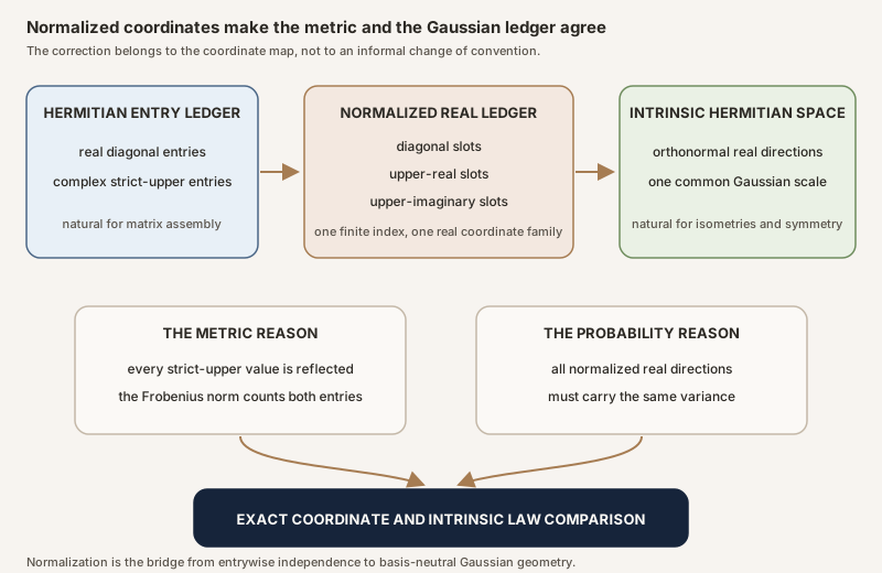
From the product law to an intrinsic Gaussian
The coordinate law first lives on a finite real function space. Mathlib’s
finite Euclidean packaging turns it into an element of
EuclideanSpace. Uniform multiplication by \(\sqrt{s_n}\) turns a
standard Gaussian into the common-variance product above.
The decoding map \(D_n\) is a real linear isometric equivalence. Standard Gaussian measure is preserved by such an isometry, so the decoded law equals an intrinsic Hermitian standard Gaussian followed by the same uniform scale:
\[ (D_n)_*\Bigl((\operatorname{WithLp.toLp}_2)_*\rho_n\Bigr) =\left(H\mapsto\sqrt{s_n}\,H\right)_* \operatorname{stdGaussian} (\operatorname{HermitianEuclidean}(n)). \]The left side first packages the finite function as Euclidean data and then decodes it. Each star denotes a pushforward measure : sample a real ledger with law \(\rho_n\), decode it, and ask for the resulting law on Hermitian matrices. The equality is a statement about complete probability distributions, not only matching means and variances.
The project then proves that the coordinate route and intrinsic route agree
entry by entry, transports both laws into ambient complex matrix space, and
obtains unitary-conjugation invariance of GUE.matrixLaw n. The
coordinate isometry is the geometric hinge in that longer proof.
Zero vector and dimension-zero policies
Two boundary cases answer different questions.
The zero vector at positive dimension. Assembly sends the zero coordinate vector to the zero matrix. Its Euclidean and Frobenius norms are both zero. Coordinate normalization remains fully defined because it never divides by the norm. Unit-vector normalization \(x/\lVert x\rVert\) is undefined at zero unless an additional convention is chosen.
Dimension zero. At \(n=0\), the diagonal and both strict-upper index sets are empty. The coordinate function space, intrinsic Hermitian space, and ambient \(0\times0\) matrix space each contain one empty zero object. Assembly and analysis are still inverse. The project sets \(s_0=0\), and the GUE law is the point mass at that unique zero matrix.
A normalized trace \(\operatorname{Tr}(H)/n\) needs its own dimension-zero policy because division by \(n\) is involved. That issue belongs to the trace observable, not to normalized Hermitian coordinates.
Boundaries that prevent common mistakes
| Tempting claim | Correct statement |
|---|---|
| “Normalized coordinates make every matrix norm one.” | They make coordinate length equal Frobenius length; the length may be any nonnegative number. |
| “Multiplying upper coordinates by \(\sqrt{2}\) changes the matrix.” | Matching decoding divides by \(\sqrt{2}\), so only the ledger changes. |
| “The four free-entry numbers already use the Frobenius metric.” | An unweighted free-entry ledger misses the conjugate-reflected copy of every upper entry. |
| “Normalized trace rescales the matrix.” | It reports the scalar \(\operatorname{Tr}(H)/n\) and leaves \(H\) unchanged. |
| “Matching coordinate variances proves equality of random-matrix laws.” | A law identity must also retain the complete joint distribution and independence structure. |
| “The map needs \(n\gt0\).” | Coordinate assembly works at \(n=0\); only operations that divide by dimension need another policy. |
| “A zero matrix breaks normalized coordinates.” | The zero ledger decodes normally; only unit-direction normalization fails at zero. |
Where to continue
Read Hermitian coordinate space for the unnormalized diagonal and complex-upper data model, Hermitian Frobenius geometry for the factor-of-two inner product, and matrix trace for the trace observable.
From Normalized Hermitian Coordinates to Gaussian Unitary Ensemble Invariance proves the isometry and follows each measure transport to the final ambient symmetry theorem. Finite GUE from Independent Gaussian Coordinates constructs the coordinate law that is later identified intrinsically.
References
Project source. GaussianUnitaryEnsembleInvariance.lean, the pinned checked definitions and theorems for the real index, inverse maps, inner-product preservation, intrinsic Gaussian comparison, and GUE invariance.
Mathlib contributors. Multivariate Gaussian distributions, real Gaussian distributions, indexed product measures, and measure maps, Mathlib 4 documentation. These official APIs support the finite product law, Gaussian scaling, standard-Gaussian transport by isometries, and composition of measurable pushforwards used by the project bridge.