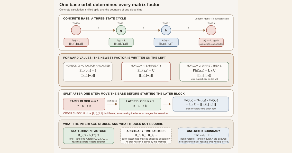
Start with three possible base states,
\[ \Omega=\{r,g,b\}, \]named red, green, and blue. Let one time step move the state around a cycle:
\[ T(r)=g, \qquad T(g)=b, \qquad T(b)=r. \]At each state, use the same rule \(A\) to select a \(2\) by \(2\) matrix:
\[ A(r)=U= \begin{bmatrix} 1&1\\ 0&1 \end{bmatrix}, \qquad A(g)=L= \begin{bmatrix} 1&0\\ 1&1 \end{bmatrix}, \qquad A(b)=I_2= \begin{bmatrix} 1&0\\ 0&1 \end{bmatrix}. \]The arithmetic is the same whether these integer entries are read as real or complex numbers. To instantiate the project’s bundled measurable cocycle, regard them as complex numbers with zero imaginary part.
The rule \(A\) is called the generator. Starting at \(r\), the base orbit and sampled factors are
\[ r\xrightarrow{T}g\xrightarrow{T}b\xrightarrow{T}r\xrightarrow{T}\cdots, \qquad U,L,I_2,U,\ldots. \]This is a small but genuine matrix cocycle example: the matrices \(U\) and \(L\) do not commute, so their order can be checked rather than ignored.
Compute the first three horizons
Write \(\Phi(k,\omega)\) for the accumulated matrix after \(k\) forward steps from state \(\omega\). A horizon counts how many matrices have acted. At horizon zero, no matrix has acted, so the value is the identity:
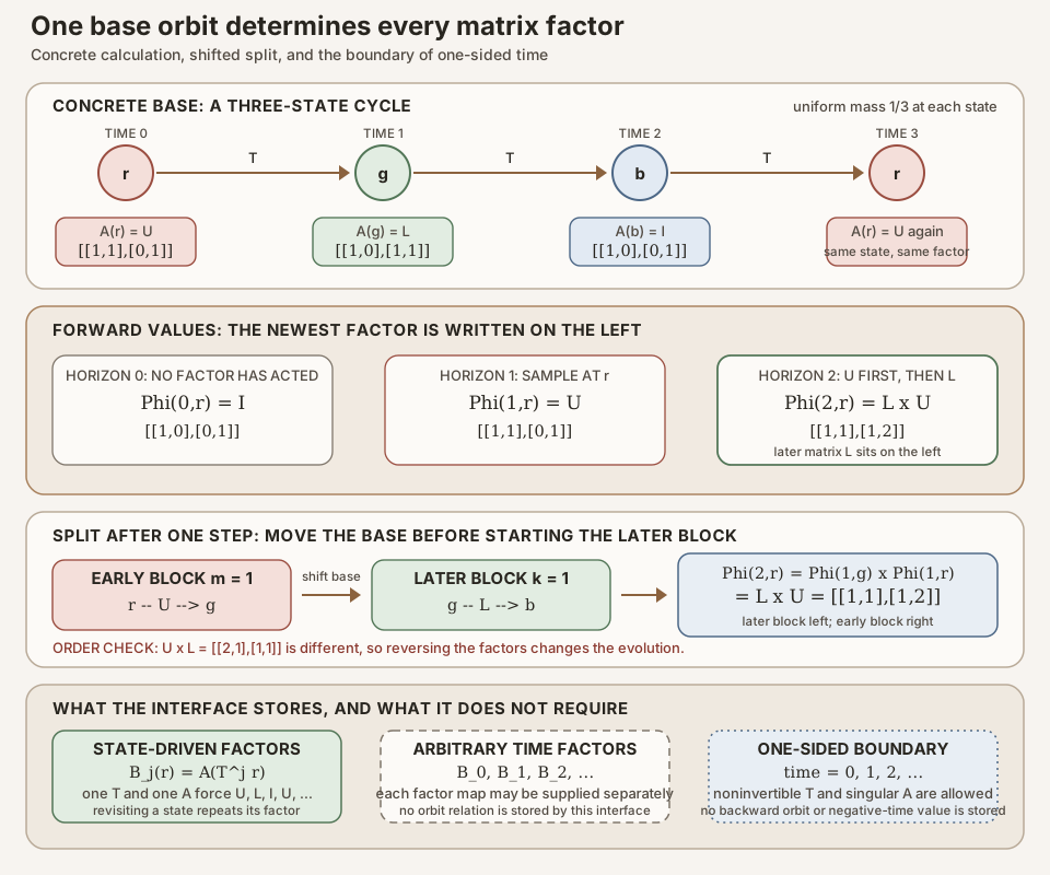
\[ \Phi(0,r)=I_2. \]At horizon one, the generator is sampled at the initial state:
\[ \Phi(1,r)=A(r)=U= \begin{bmatrix} 1&1\\ 0&1 \end{bmatrix}. \]At horizon two, \(U\) acts first and \(L\) acts second. Because matrices act on column vectors from the left, the later action is written on the left:
\[ \begin{aligned} \Phi(2,r) &=A(T(r))A(r)\\ &=LU\\ &= \begin{bmatrix} 1&0\\ 1&1 \end{bmatrix} \begin{bmatrix} 1&1\\ 0&1 \end{bmatrix}\\ &= \begin{bmatrix} 1&1\\ 1&2 \end{bmatrix}. \end{aligned} \]The reversed product is different:
\[ UL= \begin{bmatrix} 2&1\\ 1&1 \end{bmatrix} \ne \begin{bmatrix} 1&1\\ 1&2 \end{bmatrix} =LU. \]The distinction is visible on a vector. For \(v=(0,1)^{\mathsf T}\), the intended chronology gives
\[ v\xrightarrow{U} \begin{bmatrix}1\\1\end{bmatrix} \xrightarrow{L} \begin{bmatrix}1\\2\end{bmatrix}. \]That final vector is exactly \((LU)v\). Reversing the actions gives \((UL)v=(1,1)^{\mathsf T}\), a different result.
Check the cocycle identity on this orbit
Split the two-step history into an early block of \(m=1\) step and a later block of \(k=1\) step. After the early block, the base state has moved from \(r\) to \(T(r)=g\). The later block must therefore begin at \(g\):
\[ \begin{aligned} \Phi(1+1,r) &=\Phi(1,T(r))\Phi(1,r)\\ &=\Phi(1,g)\Phi(1,r)\\ &=LU\\ &= \begin{bmatrix} 1&1\\ 1&2 \end{bmatrix}. \end{aligned} \]The early block acts first and sits on the right. The shifted later block acts second and sits on the left. Omitting the shift would instead produce
\[ \Phi(1,r)\Phi(1,r)=U^2= \begin{bmatrix} 1&2\\ 0&1 \end{bmatrix}, \]which is not the two-step value. This one calculation exposes both essential conventions: shift the starting state, and preserve chronological action order.
From the example to the definition
Let \(\Omega\) be a base-state space, let \(T:\Omega\to\Omega\) advance the base by one step, and let
\[ A:\Omega\longrightarrow M_\iota(\mathbb K) \]select a square matrix at each state. Here \(\mathbb K\) is a scalar system, and \(M_\iota(\mathbb K)\) denotes matrices whose rows and columns are indexed by a finite type \(\iota\).
The \(j\)-th orbit factor is
\[ B_j(\omega)=A(T^j\omega). \]The one-sided cocycle value is the forward matrix product
\[ \Phi(k,\omega)= \begin{cases} I, & k=0,\\ A(T^{k-1}\omega)\cdots A(T\omega)A(\omega), & k\gt0. \end{cases} \]Equivalently, it is determined by the recursion
\[ \Phi(0,\omega)=I, \qquad \Phi(k+1,\omega)=A(T^k\omega)\Phi(k,\omega). \]For any natural numbers \(m\) and \(k\), splitting the history after \(m\) steps gives the one-sided cocycle identity
\[ \boxed{ \Phi(m+k,\omega)=\Phi(k,T^m\omega)\Phi(m,\omega) }. \]The project proves this law from the generator and ordered-product recursion. It does not store an unrelated two-argument function and ask the user to prove the cocycle law as a separate structure field.
State-driven factors are not arbitrary time factors
An arbitrary finite-product interface may accept independently supplied maps
\[ B_0,B_1,B_2,\ldots, \qquad B_j:\Omega\to M_\iota(\mathbb K). \]The cocycle interface in this project accepts one base map \(T\) and one generator \(A\), then forces
\[ B_j=A\circ T^j. \]In the three-state example, revisiting red forces the factor sequence along that orbit to repeat:
\[ U,L,I_2,U,L,I_2,\ldots. \]The values at different times are not separate choices. They are linked by the repeated evaluation of the same generator along one orbit. This relation is exactly what supplies the shifted state \(T^m\omega\) in the cocycle law.
This contrast is about the interface, not about what can ever be encoded. One can add time as a component of the base state and thereby represent many prescribed sequences. The present module receives its factors by evaluating one generator along an orbit, not as unrelated time-indexed inputs.
The finite random-matrix product entry develops the arbitrary-factor interface. The cocycle in this page is its orbit-generated specialization.
Why the cocycle is one-sided
The time parameter is a natural number:
\[ k\in\mathbb N=\{0,1,2,\ldots\}. \]That is what one-sided means here. The definition needs only forward iterates \(T^0,T^1,T^2,\ldots\). It never asks for \(T^{-1}\), and it never constructs \(\Phi(-1,\omega)\).
A two-sided group cocycle would require additional data and hypotheses. One would need a meaningful way to move the base backward, and matrix-valued negative-time evolution would normally require invertible finite-time values. Neither condition is hidden in this definition.
An invertible example does not create an invertibility requirement
The three-state cycle is invertible, and \(U\), \(L\), and \(I_2\) are invertible. That makes the running example convenient, but it is not a theorem about all one-sided cocycles.
For a genuinely noninvertible base, take \(\Omega=\{a,b\}\), define
\[ T(a)=a, \qquad T(b)=a, \]and put all source mass at \(a\). In other words, use the Dirac probability measure \(\delta_a\), which assigns mass one to \(a\) and mass zero to \(b\). The map \(T\) is not injective, but pushing \(\delta_a\) through \(T\) still returns \(\delta_a\), because \(a\) remains fixed. Thus \(T\) is measure preserving for this measure.
The generator at \(b\) may even be singular, for example
\[ A(b)= \begin{bmatrix} 1&0\\ 0&0 \end{bmatrix}. \]The forward values are still defined, but there is no matrix inverse for a negative-time extension from that state. The point \(b\) has measure zero under \(\delta_a\), but it is not logically absent from \(\Omega\); the null set page explains that distinction.
Measurability and measure preservation
Equip the running three-state space with the discrete collection of events , meaning every subset of \(\Omega\) is allowed. Every function out of this finite discrete measurable space is a measurable function . Therefore the base map \(T\), the generator \(A\), every factor \(\omega\mapsto A(T^j\omega)\), and every finite cocycle value are measurable.
Give the three states equal probability:
\[ \mu(\{r\})=\mu(\{g\})=\mu(\{b\})=\frac13. \]The cycle merely permutes equal-mass points, so it preserves this probability measure :
\[ T_*\mu=\mu. \]The symbol \(T_*\mu\) denotes the measure obtained by transporting \(\mu\)
through \(T\). In the general bundled Lean object, the source may be any
measure
, not necessarily one with total mass one.
The field base_preserving states both that the base is measurable
and that this pushforward equality holds.
In the general complex-matrix layer, the proof follows the same ladder:
- a measurable base has measurable natural-number iterates;
- composing a measurable generator with each iterate gives a measurable orbit factor; and
- a finite product of measurable matrix-valued functions is measurable.
Measurability answers whether preimages of matrix events are allowed events. It does not imply integrability, independence, or a probability law. This module does not push a cocycle value forward to create a law.
In Lean
Lean’s iteration notation makes the state-driven factor visible.
orbitMatrixSequence T A j ω = A (T^[j] ω)orbitMatrixSequence T Ais the time-indexed factor family built from one base map and one generator.j : ℕis the nonnegative time index.T^[j]is Lean’s syntax for the \(j\)-fold function iterate. The brackets are part of the notation; this is not a matrix power.T^[j] ωapplies that iterate to the starting stateω.A (T^[j] ω)applies the same generator to the visited state.
The exact project definition is:
def orbitMatrixSequence (T : Ω → Ω) (A : RandomMatrix Ω ι ι 𝕜) :
    ℕ → RandomMatrix Ω ι ι 𝕜 :=
  fun j ω => A (T^[j] ω)
The successor equation says aloud where the new factor goes.
cocycleProduct T A (k + 1) ω = A (T^[k] ω) * cocycleProduct T A k ωk + 1is a successor horizon. Horizon zero remains the empty product, which is the identity matrix.*is matrix multiplication here.- The newest factor appears before
*, so it acts after the value on the right when both are applied to a column vector. cocycleProduct T A k ωis the earlier \(k\)-step block from the original state.
The exact checked declaration is:
@[simp] theorem cocycleProduct_succ (T : Ω → Ω)
    (A : RandomMatrix Ω ι ι 𝕜) (k : ℕ) :
    cocycleProduct T A (k + 1) =
      fun ω => A (T^[k] ω) * cocycleProduct T A k ω := rfl
The cocycle law is the exact generalization of the \(LU\) calculation.
C.value (m + k) ω = C.value k (C.base^[m] ω) * C.value m ωCis a bundledDiscreteMatrixCocycle.C.base^[m] ωis the state reached after the early block.C.value k (C.base^[m] ω)is the later block restarted from that shifted state.- The later block is on the left of
*; the early blockC.value m ωis on the right. - The equality is pointwise at the explicitly named state
ω.
The exact theorem in the project is:
theorem value_add (C : DiscreteMatrixCocycle (ι := ι) μ)
    (m k : ℕ) (ω : Ω) :
    C.value (m + k) ω =
      C.value k (C.base^[m] ω) * C.value m ω :=
  cocycleProduct_add C.base C.generator m k ω
Finally, the bundled measurable statement reads as follows.
C.measurable_value k : Measurable (C.value k)C.value kis a function of the base state;ωis not written because Lean is asserting measurability of the whole function.Measurableis a proposition, not a probability and not an integrability bound.- Method notation
C.measurable_value kapplies the theoremDiscreteMatrixCocycle.measurable_valuetoC. - The proof uses the measurable base contained in
C.base_preservingand the separate fieldC.measurable_generator.
The exact bundled structure and proof are:
structure DiscreteMatrixCocycle (μ : Measure Ω) where
  base : Ω → Ω
  generator : RandomMatrix Ω ι ι ℂ
  base_preserving : MeasurePreserving base μ μ
  measurable_generator : Measurable generator

theorem measurable_value (C : DiscreteMatrixCocycle (ι := ι) μ) (k : ℕ) :
    Measurable (C.value k) :=
  measurable_cocycleProduct C.base C.generator
    C.base_preserving.measurable C.measurable_generator k
The algebraic product works over a semiring: a scalar system with zero, one, addition, and multiplication obeying the usual distributive laws, but not necessarily subtraction or division. The measurable bundle specializes its matrix entries to complex numbers.
Standalone tutorial
Standalone tutorial. This file imports only Lean’s
Std library. It does not import Mathlib or this project, and it
verifies the three-state orbit, the two matrix products, and the \(m=1,k=1\)
split.
Save the following as CocycleWorksheet.lean in a temporary
directory outside the repository:
import Std

namespace CocycleWorksheet

inductive State where
  | red
  | green
  | blue
deriving Repr, DecidableEq

def base : State → State
  | .red => .green
  | .green => .blue
  | .blue => .red

def baseIterate : Nat → State → State
  | 0, ω => ω
  | Nat.succ n, ω => base (baseIterate n ω)

structure Mat2 where
  a00 : Int
  a01 : Int
  a10 : Int
  a11 : Int
deriving Repr, DecidableEq

def identity : Mat2 := ⟨1, 0, 0, 1⟩
def upper : Mat2 := ⟨1, 1, 0, 1⟩
def lower : Mat2 := ⟨1, 0, 1, 1⟩

def mul (A B : Mat2) : Mat2 :=
  { a00 := A.a00 * B.a00 + A.a01 * B.a10
    a01 := A.a00 * B.a01 + A.a01 * B.a11
    a10 := A.a10 * B.a00 + A.a11 * B.a10
    a11 := A.a10 * B.a01 + A.a11 * B.a11 }

def generator : State → Mat2
  | .red => upper
  | .green => lower
  | .blue => identity

def phi : Nat → State → Mat2
  | 0, _ => identity
  | Nat.succ k, ω =>
      mul (generator (baseIterate k ω)) (phi k ω)

#eval phi 0 .red
#eval phi 1 .red
#eval phi 2 .red
#eval mul upper lower

example : phi 0 .red = identity := by decide
example : phi 1 .red = upper := by decide
example : phi 2 .red = ⟨1, 1, 1, 2⟩ := by decide

example :
    phi 2 .red =
      mul (phi 1 (baseIterate 1 .red)) (phi 1 .red) := by
  decide

end CocycleWorksheet
From that temporary directory, a human with the pinned Lean toolchain already installed can type:
elan run leanprover/lean4:v4.32.0 lean CocycleWorksheet.lean
The first four evaluations display \(I_2\), \(U\),
\(LU=\left[\begin{smallmatrix}1&1\\1&2\end{smallmatrix}\right]\), and the
reversed product
\(UL=\left[\begin{smallmatrix}2&1\\1&1\end{smallmatrix}\right]\). The final
example
is the small cocycle identity with the shifted state written explicitly. This
worksheet uses a four-field integer structure so that it stays independent of
Mathlib; it does not replace the project’s generic matrix theorems.
Try it in the repository
Full project check. This uses the repository’s pinned Lean and Mathlib
dependencies and may require substantial disk space and memory.
The authoritative source is
formalization/NonlinearDynamics/Random/RandomCocycles/Discrete.lean.
Create a
temporary probe and type:
import NonlinearDynamics.Random.RandomCocycles.Discrete

#check NonlinearDynamics.Random.RandomCocycles.orbitMatrixSequence
#check NonlinearDynamics.Random.RandomCocycles.cocycleProduct_zero
#check NonlinearDynamics.Random.RandomCocycles.cocycleProduct_succ
#check NonlinearDynamics.Random.RandomCocycles.cocycleProduct_add
#check NonlinearDynamics.Random.RandomCocycles.measurable_orbitMatrixSequence
#check NonlinearDynamics.Random.RandomCocycles.measurable_cocycleProduct
#check NonlinearDynamics.Random.RandomCocycles.DiscreteMatrixCocycle
#check NonlinearDynamics.Random.RandomCocycles.DiscreteMatrixCocycle.value_add
#check NonlinearDynamics.Random.RandomCocycles.DiscreteMatrixCocycle.measurable_value
#check NonlinearDynamics.Random.RandomCocycles.DiscreteMatrixCocycle.base_iterate_preserving
Each #check asks the pinned elaborator to display the exact type of
one checked declaration. To check the authoritative module itself, type this
literal full-project command from the repository root:
cd formalization
lake env lean NonlinearDynamics/Random/RandomCocycles/Discrete.lean
That full project check uses the repository’s pinned Lean and Mathlib dependencies and may require substantial disk space and memory.
cd formalization
lake env lean -DwarningAsError=true NonlinearDynamics/Random/RandomCocycles/Discrete.lean
Resource note: this exact file uses the repository's
pinned Lean and Mathlib dependencies. Initial project setup can require
substantial disk space and build time. For a lightweight first step on
macOS or Linux, use the page's standalone Lean-core or Std
tutorial.
Boundary cases and nonclaims
- Horizon zero: the value is the identity, not the first generator matrix.
- Empty matrix dimension: if the finite coordinate type has no elements, there is one empty square matrix. The algebraic and measurable statements remain valid; this module does not require positive dimension.
- No probability normalization:
DiscreteMatrixCocycle μaccepts a general measure. The uniform three-state probability is an example, not a structure requirement. - No independence: successive factors come from one orbit. The definition does not assert that they are independent or identically distributed.
- No invertibility: neither the base map nor the generator matrices must have inverses.
- No negative time: values are indexed by natural numbers only.
- No asymptotic theorem: finite products and their measurability do not by themselves produce Lyapunov exponents, invariant splittings, or limits.
- No integrability theorem: a measurable norm or logarithm can still have an infinite integral.
- No random-Jacobian bridge: the generator is an abstract matrix-valued map here. Identifying it with derivatives of a nonlinear system requires separate definitions and hypotheses.
Where to continue
Generator-Presented One-Sided Discrete Matrix Cocycles derives the complete checked interface and separates its algebraic, measurable, and measure-preserving layers.
Finite-Time Norm and Extended-Log-Norm Observables for Matrix Cocycles adds a concrete matrix norm and a zero-aware logarithm. That chapter is the next analytic step; it still makes no long-time multiplicative-ergodic claim.
The forward matrix product entry focuses on action order. The finite random-matrix product entry adds measurability and laws for arbitrary time-indexed factors, while the present page explains the extra orbit structure that turns those factors into a cocycle.
References
Mathlib contributors.
Function iteration,
Mathlib 4 documentation. The project uses this API for T^[j],
including its zero, successor, and addition laws.
Mathlib contributors. Measure-preserving maps, Mathlib 4 documentation. The bundled cocycle uses this API for measurability of the base, pushforward equality, and preservation by natural iterates.
Ludwig Arnold. Random Dynamical Systems, Springer Monographs in Mathematics, 1998. This develops cocycles over metric dynamical systems and their later ergodic theory. Its probability, invertibility, and asymptotic layers are not inferred on this page.
V. I. Oseledets. A multiplicative ergodic theorem. Characteristic Ljapunov exponents of dynamical systems, Transactions of the Moscow Mathematical Society 19 (1968), 197-231. This is a historical long-time destination. The finite cocycle interface here proves none of its integrability, exponent, limit, or splitting conclusions.
The exact upstream Lean source audited for this entry is Mathlib commit
81a5d257,
the revision pinned by formalization/lake-manifest.json.