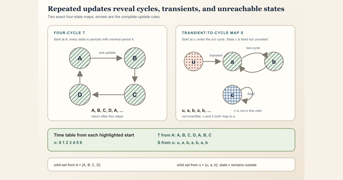
To iterate a map is to apply the same update rule repeatedly. The forward orbit of a starting state is the resulting time-ordered path, or the set of states visited along that path.
Let \(T:\Omega\to\Omega\) be a discrete-time map. Its \(n\)-th iterate is written \(T^n\), with
\[ T^0=\operatorname{id}_{\Omega}, \qquad T^{n+1}=T\circ T^n. \]For a starting state \(\omega\), the value \(T^n(\omega)\) is the state after \(n\) updates.
Start with a four-state cycle
Take the state space
\[ \Omega=\{A,B,C,D\} \]and define
\[ T(A)=B, \qquad T(B)=C, \qquad T(C)=D, \qquad T(D)=A. \]Starting at \(A\), apply the same rule one step at a time:
| Time \(n\) | \(T^n(A)\) | Reason |
|---|---|---|
| 0 | \(A\) | zero iterations leave the state unchanged |
| 1 | \(B\) | \(T(A)=B\) |
| 2 | \(C\) | \(T(T(A))=T(B)=C\) |
| 3 | \(D\) | one more update |
| 4 | \(A\) | the cycle closes |
| 5 | \(B\) | the same four-step pattern repeats |
| 6 | \(C\) | two steps into the next lap |
| 7 | \(D\) | three steps into the next lap |
| 8 | \(A\) | two complete laps |
The time-ordered forward orbit is
\[ A,B,C,D,A,B,C,D,\ldots \]and its set of visited states is
\[ \mathcal O_T^+(A) =\{T^n(A):n\in\mathbb N\} =\{A,B,C,D\}. \]The point \(A\) is periodic with minimal period four because \(T^4(A)=A\), while no positive iterate with exponent below four returns it to itself.
A transient point feeding a cycle
Now use the four-state space
\[ \Omega'=\{u,a,b,c\} \]with map \(S\) defined by
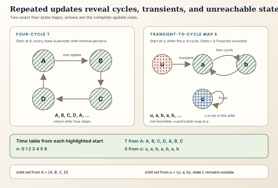
\[ S(u)=a, \qquad S(a)=b, \qquad S(b)=a, \qquad S(c)=c. \]Starting at \(u\) gives
| Time \(n\) | \(S^n(u)\) | Dynamical role |
|---|---|---|
| 0 | \(u\) | transient starting point |
| 1 | \(a\) | enters the two-cycle |
| 2 | \(b\) | other point of the cycle |
| 3 | \(a\) | first return to \(a\) |
| 4 | \(b\) | repetition continues |
| 5 | \(a\) | repetition continues |
| 6 | \(b\) | repetition continues |
Therefore
\[ \mathcal O_S^+(u)=\{u,a,b\}. \]The state \(c\) is in the state space but not in this orbit. It has its own one-point orbit \(\mathcal O_S^+(c)=\{c\}\).
The starting point \(u\) is transient because it is visited once and never revisited. The states \(a\) and \(b\) are periodic with minimal period two. The state \(c\) is fixed because \(S(c)=c\).
The next distinction is between following one orbit and controlling nearby orbits. Forward Stability asks whether every sufficiently close start remains close to this reference orbit for all natural-number times.
Iterate is not exponentiation
The notation \(T^n\) looks like a numerical power, but here it means function composition:
\[ T^3(\omega)=T\bigl(T(T(\omega))\bigr). \]Nothing is multiplied, and the state space need not contain numbers. The four-cycle uses letter-valued states and the notation works without any algebraic multiplication on \(\Omega\).
Iterates combine by addition of step counts:
\[ T^{m+n}(\omega) =T^m\bigl(T^n(\omega)\bigr). \]The expression on the right takes \(n\) steps first, then \(m\) more. The total is \(m+n\) updates.
Orbit is not state space
The state space \(\Omega\) lists every state the model permits. A forward orbit depends on a starting point and usually visits only part of that space.
In the transient example,
\[ \Omega'=\{u,a,b,c\}, \qquad \mathcal O_S^+(u)=\{u,a,b\}. \]The missing state \(c\) is not impossible; it is not reachable from \(u\) by forward iteration. A different start gives a different orbit.
It is also useful to distinguish the orbit sequence
\[ \bigl(S^n(u)\bigr)_{n\ge0}=u,a,b,a,b,\ldots \]from the orbit set \(\{u,a,b\}\). The sequence records time order and repetitions; the set discards both.
Fixed and periodic are not synonyms
A point \(\omega\) is fixed when
\[ T(\omega)=\omega. \]It is periodic when there is some positive integer \(p\) such that
\[ T^p(\omega)=\omega. \]Every fixed point is periodic with period one. A point on a genuine four-cycle is periodic but not fixed. If several positive values of \(p\) work, the smallest is called the minimal period. For \(A\) in the four-cycle, \(4,8,12, \ldots\) all return to \(A\), but the minimal period is four.
Forward iteration does not require an inverse
The forward orbit uses exponents \(n\in\mathbb N\), so it only asks how to move ahead. The map need not be injective, surjective, or invertible.
In the transient example, both \(u\) and \(b\) map to \(a\). Seeing the current state \(a\) does not determine whether the previous state was \(u\) or \(b\). There is no inverse function \(S^{-1}:\Omega'\to\Omega'\), yet every forward iterate \(S^n\) is perfectly well defined.
When \(T\) is invertible, one can additionally define a two-sided orbit indexed by integers, using negative powers for backward time. That is extra structure. The one-sided cocycles in this project deliberately require only forward time.
In Lean: square brackets mark function iteration
Lean avoids overloading ordinary numerical exponent syntax. It writes the
\(n\)-fold iterate of T as T^[n].
T^[n] ωThas function typeΩ → Ω; its input and output state types agree so the output can be fed back as the next input.^[n]is Lean’s iteration notation. The square brackets are part of the notation and distinguish function iteration from algebraic powers.n : ℕis the number of forward steps.ω : Ωis the starting state.- Function application uses spacing, so the final
ωapplies the iterated functionT^[n]to the start. T^[0] ωreduces toω, whileT^[n + 1] ωapplies one additional copy ofT.
The notation expands to Nat.iterate T n. Mathlib’s
Function.iterate_add_apply theorem is the checked rule for joining
two time blocks.
Run both finite orbits locally
A small Std-only file can execute the same repeated-update
recursion without loading Mathlib. It defines that recursion explicitly;
the exact project notation T^[n] remains in the project-backed
section below. Save this as OrbitScratch.lean in a scratch
directory outside formalization/:
import Std

def iterate {α : Type} (step : α → α) : Nat → α → α
  | 0, x => x
  | n + 1, x => step (iterate step n x)

inductive CycleState where
  | a | b | c | d
  deriving DecidableEq

def cycle4 : CycleState → CycleState
  | .a => .b
  | .b => .c
  | .c => .d
  | .d => .a

def cycleCode : CycleState → Nat
  | .a => 0
  | .b => 1
  | .c => 2
  | .d => 3

inductive TransientState where
  | u | a | b | c
  deriving DecidableEq

def transient : TransientState → TransientState
  | .u => .a
  | .a => .b
  | .b => .a
  | .c => .c

def transientCode : TransientState → Nat
  | .u => 0
  | .a => 1
  | .b => 2
  | .c => 3

#eval (List.range 9).map (fun n => cycleCode (iterate cycle4 n CycleState.a))
#eval (List.range 7).map
  (fun n => transientCode (iterate transient n TransientState.u))
#eval (List.range 4).map
  (fun n => transientCode (iterate transient n TransientState.c))

example : iterate cycle4 4 CycleState.a = CycleState.a := by decide
example : iterate transient 3 TransientState.u = TransientState.a := by decide
example : transient TransientState.u = transient TransientState.b := by decide
The codes 0, 1, 2, 3 stand for \(A,B,C,D\) in the first system
and \(u,a,b,c\) in the second. Run the file with:
source "$HOME/.elan/env"
elan run leanprover/lean4:v4.32.0 lean OrbitScratch.lean
This exact worksheet was executed successfully with Lean 4.32.0 and printed:
[0, 1, 2, 3, 0, 1, 2, 3, 0]
[0, 1, 2, 1, 2, 1, 2]
[3, 3, 3, 3]
The first two lines reproduce both orbit tables. The third checks that
\(c\) is fixed. The last proposition records the noninvertibility witness:
different states \(u\) and \(b\) have the same image \(a\). This file is small
enough for a normal Mac or Linux machine because it imports only
Std. The matrix-valued, measurable project interface still
requires the full project check below.
Exact project usage: sampling a matrix along an orbit
The one-sided cocycle module uses the iterate directly. This is its exact checked definition:
def orbitMatrixSequence (T : Ω → Ω) (A : RandomMatrix Ω ι ι 𝕜) :
    ℕ → RandomMatrix Ω ι ι 𝕜 :=
  fun j ω => A (T^[j] ω)
For a time j and start ω, Lean first computes the orbit
state T^[j] ω, then evaluates matrix generator A there.
The definition is finite and pointwise. It assumes no measure, probability,
ergodicity, invertibility, or limiting behavior.
The same module proves measurability at every finite iterate:
theorem measurable_orbitMatrixSequence (T : Ω → Ω)
    (A : RandomMatrix Ω ι ι ℂ) (hT : Measurable T) (hA : Measurable A)
    (j : ℕ) : Measurable (orbitMatrixSequence T A j) :=
  hA.comp (hT.iterate j)
The theorem states that a measurable map remains measurable after a finite number of iterations, and composing the measurable generator with that iterate stays measurable. It does not state that the map preserves a measure; that is a separate property.
The authoritative checked source is
formalization/NonlinearDynamics/Random/RandomCocycles/Discrete.lean.
A human can type this worksheet in a scratch buffer inside a clone with the
repository’s pinned dependencies installed:
import NonlinearDynamics.Random.RandomCocycles.Discrete

open Function
open NonlinearDynamics.Random.RandomCocycles

#check Nat.iterate
#check Function.iterate_zero_apply
#check Function.iterate_succ_apply
#check Function.iterate_add_apply
#check orbitMatrixSequence
#check measurable_orbitMatrixSequence

inductive TutorialState where
  | a | b | c | d

open TutorialState

def cycle4 : TutorialState → TutorialState
  | a => b
  | b => c
  | c => d
  | d => a

example : cycle4^[0] a = a := by rfl
example : cycle4^[4] a = a := by rfl
example : cycle4^[5] a = b := by rfl

example {Ω : Type*} (T : Ω → Ω) (m n : ℕ) (ω : Ω) :
    T^[m + n] ω = T^[m] (T^[n] ω) :=
  Function.iterate_add_apply T m n ω
The custom four-state type makes the first mathematical example executable.
The three rfl proofs reduce the finite iterate exactly. The final
example checks the rule for concatenating two time blocks. The full-project command
below checks the complete project module containing the orbit-sampling
definition and measurability theorem.
cd formalization
lake env lean -DwarningAsError=true NonlinearDynamics/Random/RandomCocycles/Discrete.lean
Resource note: this exact file uses the repository's
pinned Lean and Mathlib dependencies. Initial project setup can require
substantial disk space and build time. For a lightweight first step on
macOS or Linux, use the page's standalone Lean-core or Std
tutorial.
Boundaries that prevent common mistakes
| Tempting shortcut | Correct statement |
|---|---|
| “\(T^n\) multiplies \(T\) by itself.” | It composes a self-map with itself \(n\) times. |
| “The orbit is the state space.” | The orbit is the part reached from one start; other allowed states can be absent. |
| “Periodic means fixed.” | Fixed means period one; a periodic point may have larger minimal period. |
| “An orbit is just a set.” | The orbit sequence retains order and repetitions; the orbit set discards both. |
| “Iteration requires invertibility.” | Forward natural-number iteration works for any self-map. |
| “A finite orbit proves measure preservation or ergodicity.” | Those are separate measure-theoretic properties of the map. |
Where to continue
The event entry explains how a set can ask whether an orbit state has entered a region. The Birkhoff sum entry samples an observable at the finite orbit points \(\omega,T\omega,T^2\omega,\ldots\) and adds those readings. The basin of attraction instead collects starting states according to the limit of their full forward orbits.
For the matrix-valued use of forward orbits, continue to Generator-Presented One-Sided Discrete Matrix Cocycles. That chapter builds finite matrix products along the orbit while keeping one-sidedness, product order, measurability, and measure preservation separate.
References
Mathlib contributors.
Function iteration,
Mathlib 4 documentation. This official source defines T^[n] and
the zero, successor, addition, and multiplication laws for iterates.
Mathlib contributors. Periodic points, Mathlib 4 documentation. This official source defines fixed points, periodic points, minimal periods, and finite periodic orbits.
Project source. Discrete.lean contains the checked orbit-matrix sequence and finite one-sided cocycle interfaces used in the Lean section.