Start with a three-state orbit
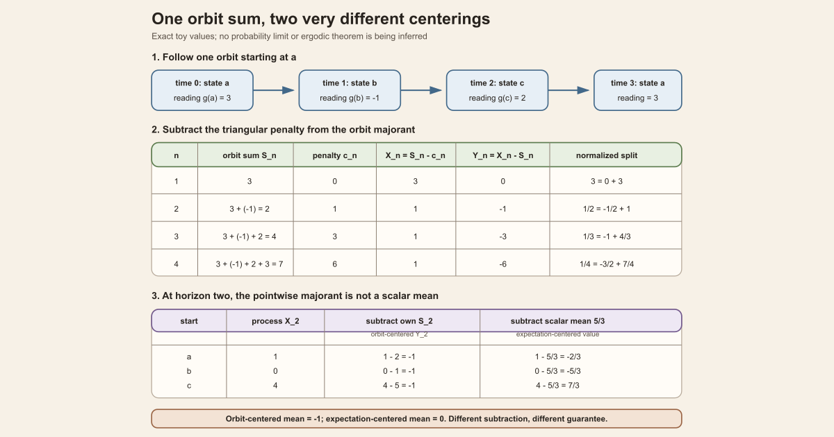
Take the finite state space \(\Omega=\{a,b,c\}\). Let one time step move cyclically,
\[ T(a)=b,\qquad T(b)=c,\qquad T(c)=a, \]and attach the one-step readings
\[ g(a)=3,\qquad g(b)=-1,\qquad g(c)=2. \]Starting at \(a\), the readings are \(3,-1,2,3,\ldots\). Their first \(n\)-term orbit sum is
\[ S_n(\omega)=\sum_{j=0}^{n-1}g(T^j\omega). \]Now subtract the triangular penalty
\[ c_n=\frac{n(n-1)}2 \]and define a finite-time process
\[ X_n(\omega)=S_n(\omega)-c_n. \]This is a real, checkable example of a shifted-subadditive process. That phrase means that the value over a combined time interval is at most the value over the first interval plus the value over the shifted second interval:
\[ X_{m+n}(\omega) \le X_m(\omega)+X_n(T^m\omega). \]Indeed, orbit sums split exactly, while
\[ c_{m+n}=c_m+c_n+mn. \]Therefore
\[ X_m(\omega)+X_n(T^m\omega)-X_{m+n}(\omega)=mn\ge0. \]The nonnegative number \(mn\) is the visible slack in the inequality. No measure, probability, limit, or integrability argument is hiding in this calculation.
Compute the majorant and remainder
The one-step value of this process is
\[ X_1(\omega)=S_1(\omega)-c_1=g(\omega). \]So the orbit sum of \(X_1\) is exactly \(S_n\). It is a majorant, or pointwise upper bound, because
\[ X_n(\omega)=S_n(\omega)-c_n\le S_n(\omega). \]Orbit-majorant centering subtracts that upper bound:
\[ Y_n(\omega)=X_n(\omega)-S_n(\omega)=-c_n. \]At the starting state \(a\), every term can be checked by hand:
| Horizon \(n\) | Readings used | Orbit majorant \(S_n(a)\) | Penalty \(c_n\) | Process \(X_n(a)\) | Centered \(Y_n(a)\) | Normalized split |
|---|---|---|---|---|---|---|
| 0 | none | 0 | 0 | 0 | 0 | totalized boundary: \(0=0+0\) |
| 1 | \(3\) | 3 | 0 | 3 | 0 | \(3=0+3\) |
| 2 | \(3,-1\) | 2 | 1 | 1 | -1 | \(1/2=-1/2+1\) |
| 3 | \(3,-1,2\) | 4 | 3 | 1 | -3 | \(1/3=-1+4/3\) |
| 4 | \(3,-1,2,3\) | 7 | 6 | 1 | -6 | \(1/4=-3/2+7/4\) |
The normalized column checks the identity
\[ \frac{X_n(\omega)}n {} = \frac{Y_n(\omega)}n+\frac{S_n(\omega)}n \]at several positive horizons. The last summand is the finite Birkhoff average of the one-step observable. The identity is arithmetic; it does not say that any term has a limit.
Why this is not expectation centering
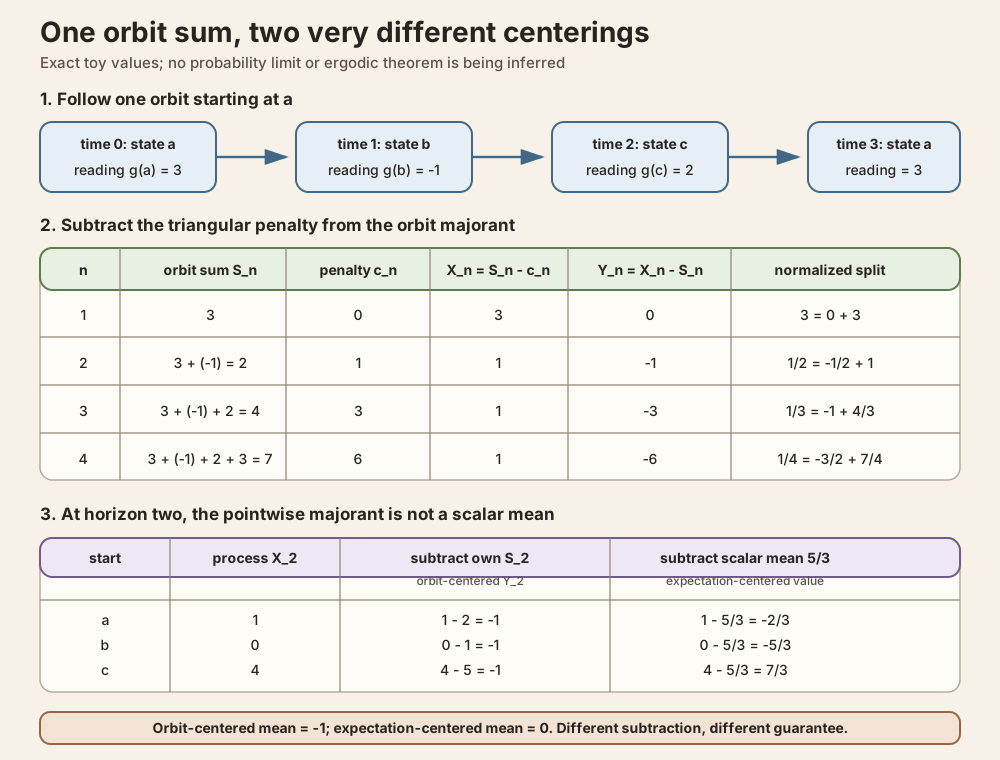
Put the uniform probability measure on the three states, so each state has probability \(1/3\). An expectation is then the ordinary average of the three values. At horizon two,
\[ X_2(a)=1,\qquad X_2(b)=0,\qquad X_2(c)=4, \]and hence
\[ \mathbb E[X_2]=\frac{1+0+4}{3}=\frac53. \]Expectation centering subtracts this one scalar from every sample:
\[ \begin{array}{c|ccc} \omega&a&b&c\\ \hline X_2(\omega)-\mathbb E[X_2]&-\frac23&-\frac53&\frac73. \end{array} \]Those three values average to zero, but one is positive. Orbit-majorant centering subtracts the sample-dependent orbit sums \(S_2(a)=2\), \(S_2(b)=1\), and \(S_2(c)=5\), giving
\[ Y_2(a)=Y_2(b)=Y_2(c)=-1. \]These values are pointwise nonpositive, but their expectation is \(-1\), not zero. The two operations solve different problems:
| Operation | Quantity subtracted | Conclusion for this example |
|---|---|---|
| orbit-majorant centering | \(S_n(\omega)\), which depends on the sample and horizon | \(Y_n(\omega)\le0\), with shifted subadditivity preserved |
| expectation centering | the scalar \(\mathbb E[X_n]\) | the centered values have expectation zero |
| time normalization | division by positive \(n\) | values are expressed per step |
Expectation centering requires a measure and enough integrability to define the expectation. Orbit-majorant centering is finite pointwise algebra and needs neither. Merely subtracting a different expected value at each horizon also does not preserve the original pointwise subadditive inequality automatically.
The general construction
Let \(\Omega\) be any state space, let \(T:\Omega\to\Omega\) advance the state by one time step, and let \(X:\mathbb N\to\Omega\to\mathbb R\) be a process. Its one-step orbit sum is
\[ \operatorname{BSum}(T,X_1,n,\omega) {} = \sum_{j=0}^{n-1}X_1(T^j\omega). \]Mathlib’s finite definition and its exact addition law supply this algebra (official documentation, pinned source).
The project defines
\[ \operatorname{Center}(T,X,n,\omega) {} = X_n(\omega)-\operatorname{BSum}(T,X_1,n,\omega). \]The name orbit-majorant centering is project terminology. It records both
the orbit sum being subtracted and the theorem that this sum bounds a
shifted-subadditive process at positive horizons. In Lean, the definition
itself is more neutrally named centeredProcess.
In Lean: define the centered process
centeredProcess T X n ωTis the one-step self-map.X n ωis the original finite-time value at horizonnand sampleω.X 1is the function \(\omega\mapsto X_1(\omega)\).birkhoffSum T (X 1) n ωadds that function over indices0, …, n - 1.centeredProcesssubtracts the finite sum. The definition does not mention a measure or an expectation.
The exact project definition is:
def centeredProcess {Ω : Type uΩ} (T : Ω → Ω) (X : ℕ → Ω → ℝ)
    (n : ℕ) (ω : Ω) : ℝ :=
  X n ω - birkhoffSum T (X 1) n ω
In Lean: use the one-step majorant
hX.oneStepBirkhoffMajorant_of_ne_zero n hn ωhXpackages the shifted-subadditive law and finite-horizon integrability forX.hn : n ≠ 0records the positive-horizon boundary without converting the natural number to an ordered scalar.oneStepBirkhoffMajorantis the all-horizon variant. It also asks forhX0 : X 0 = 0.- The proof of this inequality uses only
hX.add_le. The structure contains integrability, but the pointwise induction does not use it.
Subtracting the upper bound proves
centeredProcess T X n ω ≤ 0 for n ≠ 0. The additive
splitting law for birkhoffSum also proves that the centered family
remains shifted-subadditive.
In Lean: split the normalized value
normalized_eq_centered_add_birkhoffAverage n ω- The theorem is an equality, not a convergence assertion.
birkhoffAverage ℝ T (X 1) n ωis the real-valued orbit sum scaled by the inverse of the natural-number cast ofn.- The pinned average definition makes that scaling explicit (source).
- Lean’s real division is total at
n = 0. The theorem then reduces to0 = 0 + 0; it does not recoverX 0 ωor justify informal division by zero. - No measurable space, measure, preservation, probability, or ergodicity parameter occurs in this identity.
A tiny standalone Lean/Std worksheet
Standalone tutorial. This complete file reproduces the
three-state arithmetic with integers and exact rational numbers. It imports
Std, not Mathlib or this repository. Save it as
OrbitMajorantTutorial.lean in a scratch directory.
import Std

namespace OrbitMajorantTutorial

inductive State where
  | a | b | c
deriving Repr, DecidableEq

def step : State → State
  | .a => .b
  | .b => .c
  | .c => .a

def reading : State → Int
  | .a => 3
  | .b => -1
  | .c => 2

def iterate : Nat → State → State
  | 0, x => x
  | n + 1, x => iterate n (step x)

def orbitSum : Nat → State → Int
  | 0, _ => 0
  | n + 1, x => orbitSum n x + reading (iterate n x)

def penalty : Nat → Nat
  | 0 => 0
  | n + 1 => penalty n + n

def process (n : Nat) (x : State) : Int :=
  orbitSum n x - Int.ofNat (penalty n)

def centered (n : Nat) (x : State) : Int :=
  process n x - orbitSum n x

def normalized (z : Int) (n : Nat) : Rat :=
  (z : Rat) / (n : Rat)

def states : List State := [.a, .b, .c]

def processMean (n : Nat) : Rat :=
  let total : Int := states.foldl (fun s x => s + process n x) 0
  (total : Rat) / 3

def expectationCentered (n : Nat) (x : State) : Rat :=
  (process n x : Rat) - processMean n

def subadditiveSlack (m n : Nat) (x : State) : Int :=
  process m x + process n (iterate m x) - process (m + n) x

#eval (List.range 5).map (fun n => orbitSum n .a)
#eval (List.range 5).map (fun n => process n .a)
#eval (List.range 5).map (fun n => centered n .a)
#eval states.map (fun x => process 2 x)
#eval states.map (expectationCentered 2)

example : (List.range 5).map (fun n => orbitSum n .a) =
    [0, 3, 2, 4, 7] := by decide

example : (List.range 5).map (fun n => centered n .a) =
    [0, 0, -1, -3, -6] := by decide

example : subadditiveSlack 2 3 .b = 6 := by decide

example : normalized (process 4 .a) 4 = (1 : Rat) / 4 := by native_decide

example : normalized (process 4 .a) 4 =
    normalized (centered 4 .a) 4 + normalized (orbitSum 4 .a) 4 := by
  native_decide

example : states.map (expectationCentered 2) =
    [(-2 : Rat) / 3, (-5 : Rat) / 3, (7 : Rat) / 3] := by native_decide

end OrbitMajorantTutorial
From the directory containing the file, a human types:
source "$HOME/.elan/env"
elan run leanprover/lean4:v4.32.0 lean OrbitMajorantTutorial.lean
This exact worksheet was executed successfully with Lean 4.32.0 while editing
this page. Its first three outputs were [0, 3, 2, 4, 7],
[0, 3, 1, 1, 1], and [0, 0, -1, -3, -6]. The next
output was [1, 0, 4]; the final output displayed
[(-2 : Rat)/3, (-5 : Rat)/3, (7 : Rat)/3]. The integer examples
use decide, while the rational equalities deliberately use
native_decide so Lean evaluates normalized rational arithmetic.
This bounded worksheet is suitable for an ordinary Mac or Linux machine.
Try the exact declarations in the project
Full project check. This uses the repository’s pinned Lean and Mathlib dependencies and may require substantial disk space and memory. Create a query file containing:
import NonlinearDynamics.Random.RandomCocycles.SubadditiveCentering

open NonlinearDynamics.Random.RandomCocycles

#check centeredProcess
#check centeredProcess_zero
#check centeredProcess_one
#check IsIntegrableSubadditiveProcessCandidate.oneStepBirkhoffMajorant_of_ne_zero
#check IsIntegrableSubadditiveProcessCandidate.oneStepBirkhoffMajorant
#check IsIntegrableSubadditiveProcessCandidate.centeredProcess_nonpos_of_ne_zero
#check IsIntegrableSubadditiveProcessCandidate.centeredProcess_nonpos
#check IsIntegrableSubadditiveProcessCandidate.centeredProcess_add_le
#check IsIntegrableSubadditiveProcessCandidate.integrable_centeredProcess
#check IsIntegrableSubadditiveProcessCandidate.centeredProcess_candidate
#check normalized_eq_centered_add_birkhoffAverage
#check DiscreteMatrixCocycle.centeredLogPlusNormObservable
#check DiscreteMatrixCocycle.centeredLogPlusNormObservable_nonpos
#check DiscreteMatrixCocycle.centeredLogPlusNormObservable_add_le
Each #check asks the pinned elaborator for an exact declaration
type. The full-project command below checks the authoritative module, including its
Mathlib imports, with the repository’s pinned Lean and Mathlib dependencies
installed.
cd formalization
lake env lean -DwarningAsError=true NonlinearDynamics/Random/RandomCocycles/SubadditiveCentering.lean
Resource note: this exact file uses the repository's
pinned Lean and Mathlib dependencies. Initial project setup can require
substantial disk space and build time. For a lightweight first step on
macOS or Linux, use the page's standalone Lean-core or Std
tutorial.
Boundary cases and assumption ledger
| Claim | Premise doing the work | Important boundary |
|---|---|---|
| define \(Y_n\) | finite subtraction | no measure is needed |
| \(Y_n\le0\) for \(n\ne0\) | shifted subadditivity | no time-zero normalization is needed |
| \(Y_n\le0\) for every \(n\) | shifted subadditivity and \(X_0=0\) | a general process may retain positive \(X_0\) |
| shifted subadditivity of \(Y\) | additivity of the orbit sum | no probability or ergodicity is needed |
| integrability of every \(Y_n\) | integrability of \(X_n\) and preservation by \(T\) | composition needs an analytic transport theorem |
| normalized splitting | real arithmetic | at \(n=0\) the totalized equality is only \(0=0\) |
The time-zero premise is genuinely necessary for a uniform sign theorem. The constant process \(X_n(\omega)=1\) is shifted-subadditive because \(1\le1+1\), but its centered time-zero value is \(Y_0(\omega)=X_0(\omega)=1\). At one step, by contrast, \(Y_1=X_1-X_1=0\) for every process.
The word majorant is also narrow. It says that the orbit sum lies above \(X_n\) at the same sample and horizon. It does not say the bound is close, least possible, or bounded away from \(-\infty\) after subtraction. In the worked example the negative gap grows quadratically.
Matrix-cocycle specialization
For a discrete matrix cocycle, the project applies the same construction to
the finite-time log-positive norm observable. Its one-step Birkhoff sum is the
already defined orbitLogPlusSum. The resulting
centeredLogPlusNormObservable is pointwise nonpositive and remains
shifted-subadditive. The hypothesis
HasIntegrableGeneratorLogPlus enters only when the result promises
an integrable process candidate.
This specialization still uses a log-positive envelope. It records expansion above norm one and deliberately discards signed contraction. A centered log-positive remainder is not a signed Lyapunov exponent.
What this term does not claim
Orbit-majorant centering establishes finite algebra. By itself it does not establish:
- expectation zero or statistical unbiasedness;
- a lower bound or absolute-value bound for the centered process;
- convergence pointwise, almost everywhere, in probability, in distribution, or in \(L^1\);
- convergence of the Birkhoff average in the normalized identity;
- Birkhoff’s pointwise ergodic theorem or Kingman’s subadditive ergodic theorem;
- equality between a samplewise limit and an integrated growth rate;
- permission to exchange a limit and an integral;
- probability normalization, ergodicity, independence, mixing, or decay of correlations; or
- a signed logarithmic growth rate, Lyapunov exponent, or Oseledets splitting.
The finite reduction is one ingredient in standard routes toward subadditive ergodic theorems. The later limit arguments require their own hypotheses and proofs (Karlsson and Margulis, Lalley).
Where to continue
The Birkhoff sum entry develops the finite sum, its indexing, and its addition law. The phase averaging entry uses the centered remainder in the next finite block estimate.
The Development Notebook maps the declarations to their checked proof architecture. The full Deep Dive develops the longer route toward subadditive ergodic theory. Both are public working notes and remain distinct from this glossary definition.
References
Mathlib contributors. Birkhoff sums, Mathlib 4 documentation. This official page defines the finite orbit sum and states its zero, one, successor, and addition laws.
Mathlib contributors.
Pinned Birkhoff-sum source,
Mathlib commit 81a5d257. These lines define
birkhoffSum and prove the finite identities used by the project.
Mathlib contributors.
Pinned Birkhoff-average source,
Mathlib commit 81a5d257. The source defines normalization by the
inverse natural-number cast and proves that the zero-time average is zero.
Anders Karlsson and Gregory A. Margulis. A Multiplicative Ergodic Theorem and Nonpositively Curved Spaces, Communications in Mathematical Physics 208(1), 107-123, 1999, doi:10.1007/s002200050750. On printed page 117, the proof subtracts the additive one-step orbit cocycle from a general subadditive cocycle before later ergodic arguments.
Steven P. Lalley. Kingman’s Subadditive Ergodic Theorem, lecture notes, 3 pages, accessed 2026-07-21. Page 1 writes the same one-step subtractive reduction and uses Birkhoff’s theorem only later.
The exact upstream Mathlib revision audited for this entry is commit
81a5d257,
the v4.32.0 revision pinned by
formalization/lake-manifest.json.