Start with one orbit, the sequence of states
\[ \omega,\ T\omega,\ T^2\omega,\ T^3\omega,\ldots \]obtained by repeatedly applying a map \(T\). The notation \(T^k\omega\) means “apply \(T\) exactly \(k\) times to the starting state \(\omega\).” See orbit and iterate for that basic language.
Suppose the observable \(g\) writes the next positive integer at the \(k\)-th orbit start:
\[ g(T^k\omega)=k+1. \]We want the finite orbit sum through start \(11\):
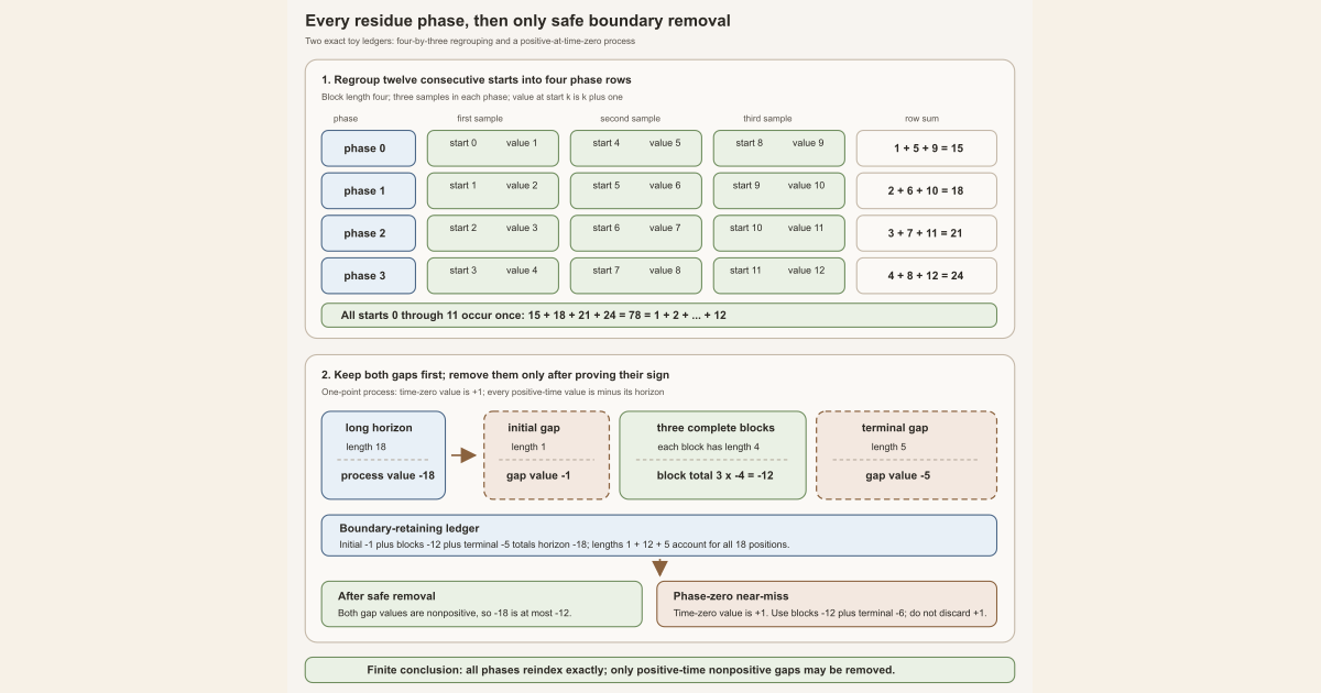
\[ 1+2+\cdots+12=78. \]Now deliberately scramble those twelve terms. Choose block length \(b=4\) and take \(q=3\) samples in each phase. A phase is one offset inside a block, so the four phases are \(s=0,1,2,3\). Within one phase, advance four orbit steps at a time:
| Phase \(s\) | Orbit starts \(4j+s\), for \(j=0,1,2\) | Observed values | Row sum |
|---|---|---|---|
| \(0\) | \(0,4,8\) | \(1,5,9\) | \(15\) |
| \(1\) | \(1,5,9\) | \(2,6,10\) | \(18\) |
| \(2\) | \(2,6,10\) | \(3,7,11\) | \(21\) |
| \(3\) | \(3,7,11\) | \(4,8,12\) | \(24\) |
Adding the rows gives
\[ 15+18+21+24=78. \]Every start from \(0\) through \(11\) appears exactly once. Grouping by phase changed the order of addition, not the terms being added.
Here is the nearest failure: keeping only phase \(0\) gives \(15\), not \(78\). The identity needs every residue phase \(0\le s\lt b\). Repeating one phase would duplicate some starts; omitting one would leave holes.
What phase averaging means
Phase averaging is a deterministic finite-sum method. Choose a block length, write one fixed-block estimate for every offset inside that block, add the estimates, and only then divide by the number of phases when that number is positive.
The word averaging is narrow here:
- no phase is selected at random;
- no expectation is taken;
- no time horizon tends to infinity; and
- no theorem about convergence is hidden in the notation.
The construction follows orbit-majorant centering . Centering supplies a shifted-subadditive process whose values are nonpositive at every positive horizon. Phase averaging uses that sign to remove two finite boundary gaps. It then uses an exact reindexing to replace a rectangle of fixed-block samples by one ordinary Birkhoff sum , meaning a finite sum along consecutive orbit iterates.
The general finite reindexing
Let \(\Omega\) be a state space, let \(T:\Omega\to\Omega\) be a self-map, and let \(g:\Omega\to M\) take values in an additive commutative monoid \(M\). That algebraic phrase means that the values have a zero, addition is associative, and finite sums may be reordered.
Let \(b,q\in\mathbb N\), where \(\mathbb N\) is the set of nonnegative whole numbers:
- \(b\) is the block length and the number of residue phases;
- \(q\) is the number of samples in each phase; and
- \(s\), with \(0\le s\lt b\), is the offset that labels one phase.
The phase-\(s\) sum is
\[ \begin{aligned} B_s(\omega) &=\operatorname{BSum}\!\left(T^b,g,q,T^s\omega\right) \\ &=\sum_{j=0}^{q-1}g\!\left(T^{bj+s}\omega\right). \end{aligned} \]The first input \(T^b\) says that successive samples in this row are \(b\) ordinary orbit steps apart. The starting state \(T^s\omega\) chooses the phase.
Every natural number \(k\lt bq\) has a unique quotient-remainder form
\[ k=bj+s, \qquad j\lt q, \qquad s\lt b. \]Therefore the rectangular grid and the consecutive orbit sum contain exactly the same terms:
\[ \boxed{ \sum_{s=0}^{b-1} \operatorname{BSum}\!\left(T^b,g,q,T^s\omega\right) {} = \operatorname{BSum}(T,g,bq,\omega). } \]This is equality, not an approximation. It needs no measure assigning weights to sets, no probability law , no measurability , no integrability , no preservation property, and no ergodicity . It is a theorem about finite sums and natural-number indices. Commutativity matters: the left side groups by phase, while the right side orders by orbit time. Order-sensitive noncommutative products need a different statement.
Mathlib’s finite Birkhoff-sum laws and function-iterate laws supply the upstream bookkeeping (official Birkhoff-sum documentation, pinned Birkhoff source, pinned iterate source).
In Lean: reindex the whole phase grid
sum_phase_birkhoffSum T g b q ωsum_phase_birkhoffSumis the checked theorem name.Tis the original map andgis the observable.bis both the iterate stride and the number of phases.qis the number of entries in each phase row.ωis the starting state.- In the theorem’s displayed type,
Finset.range bis the finite set \(0,1,\ldots,b-1\),∑adds over it, andT^[s]is Lean syntax for the \(s\)-fold iterate \(T^s\). - The invisible typeclass
[AddCommMonoid M]records exactly the algebra needed to regroup the finite sum.
The exact declaration is more informative than a call site because it shows the weak assumptions:
theorem sum_phase_birkhoffSum
    {M : Type*} [AddCommMonoid M] {Ω : Type*}
    (T : Ω → Ω) (g : Ω → M) (b q : ℕ) (ω : Ω) :
    ∑ s ∈ Finset.range b,
        birkhoffSum (T^[b]) g q (T^[s] ω) =
      birkhoffSum T g (b * q) ω
A numeric boundary process, including the time-zero trap
The reindexing identity does not yet compare a long-horizon subadditive value with the block rows. For that comparison, use a second exact example.
Take a state space with one point, let \(T\) be the identity map, and define
\[ X_0=1, \qquad X_n=-n\quad\text{for }n\gt0. \]This process is shifted-subadditive, meaning
\[ X_{m+n}(\omega) \le X_n(T^m\omega)+X_m(\omega). \]When \(m,n\gt0\), equality holds because
\[ -(m+n)=(-n)+(-m). \]If either index is zero, the \(X_0=1\) on the right only makes the inequality easier to satisfy. Thus this is a real example in which every positive-time value is nonpositive but the time-zero value is positive.
Choose \(b=4\), \(q=3\), terminal parameter \(r=2\), and phase \(s=1\). The theorem’s horizon is
\[ N=bq+b+r=4\cdot3+4+2=18. \]The phase-one decomposition has:
- an initial gap of length \(1\), contributing \(X_1=-1\);
- three complete blocks of length \(4\), contributing \(3X_4=3(-4)=-12\); and
- a terminal gap of length \(b+r-s=5\), contributing \(X_5=-5\).
The boundary-retaining estimate is equality in this model:
\[ X_{18}=-18 {} = -12-5-1. \]Both gap values are nonpositive, so discarding them increases the right side:
\[ X_{18}=-18\le-12. \]The near-miss is phase \(s=0\). A careless proof might insert \(X_0\) and then discard it, but \(X_0=1\gt0\). That inference is invalid. The checked proof instead starts directly with three complete blocks and the length-six terminal gap:
\[ X_{18} \le 3X_4+X_6 {} = -12-6 {} = -18. \]It never needs a sign hypothesis at time zero.
The general boundary geometry
Let \(X_n(\omega)\) be any real-valued shifted-subadditive process. Fix \(b,q,r\in\mathbb N\) and use the exact horizon
\[ N=bq+b+r. \]The terminal parameter \(r\) is unrestricted; the theorem does not assume \(r\lt b\). For any phase \(s\lt b\), natural-number arithmetic gives
\[ N=s+bq+(b+r-s). \]The three pieces are an initial gap of length \(s\), \(q\) complete blocks of length \(b\), and a terminal gap of length \(b+r-s\). Repeated shifted-subadditivity gives
\[ \begin{aligned} X_N(\omega)\le{}& \operatorname{BSum}\!\left(T^b,X_b,q,T^s\omega\right) \\ &+X_{b+r-s}\!\left(T^{bq+s}\omega\right) +X_s(\omega). \end{aligned} \]The condition \(s\lt b\) ensures \(b+r-s\ge1\), so the terminal gap is strictly positive even when \(r=0\).
In Lean: retain every boundary term
hX.le_phase_birkhoffSum_add_boundaries b q r s hs ωhXis a bundledIsIntegrableSubadditiveProcessCandidate T μ X. Itsadd_lefield is the shifted-subadditive inequality.b q r sare the block length, blocks per phase, terminal parameter, and phase.hs : s < bcertifies that \(s\) is a valid phase. The symbol<is the ordinary strict order on natural numbers.T^[s] ωis the shifted starting point \(T^s\omega\).(T^[b])^[q]advances \(q\) times by the powered map \(T^b\), which reaches \(T^{bq}\).- The proof uses
hX.add_le; the theorem remains stated for the full candidate structure, including its measurability and integrability fields.
This theorem keeps both boundary values visible. No sign assumption has been used yet.
Positive-time nonpositivity removes the gaps
Now assume
\[ n\ne0 \quad\Longrightarrow\quad X_n(\omega)\le0 \]for every state \(\omega\). For \(0\lt s\lt b\), both gap lengths are positive, so both boundary values are nonpositive and may be removed from an upper bound:
\[ X_N(\omega) \le \operatorname{BSum}\!\left(T^b,X_b,q,T^s\omega\right). \]For \(s=0\), the proof takes the separate direct route shown in the numeric example. This case split is why the theorem requires no claim about \(X_0\).
In Lean: remove only positive-time gaps
hX.le_phase_birkhoffSum hnonpos b q r s hs ωhnonposhas exact type∀ n, n ≠ 0 → ∀ ω, X n ω ≤ 0. The proof must supplyn ≠ 0before using the sign.le_phase_birkhoffSumis the boundary-dropping theorem, distinct from the preceding boundary-retaining theorem.hsproves \(s\lt b\). It also implies that a phase exists only when \(b\gt0\).The conclusion is pointwise at the explicit state
ω, meaning it gives a separate inequality for each starting state. There is noalmost-everywhere quantifier and no limit.
Sum first, divide only for a positive block length
The left side of the phase bound is the same for every \(s\lt b\). Summing all \(b\) inequalities gives
\[ b\,X_{bq+b+r}(\omega) \le \sum_{s=0}^{b-1} \operatorname{BSum}\!\left(T^b,X_b,q,T^s\omega\right). \]Apply the exact phase-grid reindexing to the right side:
\[ \boxed{ b\,X_{bq+b+r}(\omega) \le \operatorname{BSum}(T,X_b,bq,\omega). } \]This multiplication form remains a valid total statement at \(b=0\). If \(b\ne0\), then \(b\gt0\), so division preserves the inequality:
\[ \boxed{ X_{bq+b+r}(\omega) \le \frac{1}{b}\operatorname{BSum}(T,X_b,bq,\omega). } \]This last expression is the literal arithmetic average of the \(b\) phase inequalities. It is neither a random expectation nor an asymptotic Birkhoff average.
In Lean: keep multiplication total, then divide with evidence
hX.natCast_mul_le_birkhoffSum_phase_average hnonpos b q r ωnatCastin the theorem name records that the natural number \(b\) is cast to a real number before multiplying the real value \(X_N\).mulrecords the multiplication form; this version does not needb ≠ 0.birkhoffSum T (X b) (b * q) ωsums the block observableX bat the first \(bq\) consecutive starts of the original map.- The theorem is finite and pointwise. Its name does not imply a limiting average.
For the division form, the extra evidence is explicit:
hX.le_birkhoffSum_phase_average_div hnonpos b q r hb ωhb : b ≠ 0proves that the denominator is positive after the natural number is cast to \(\mathbb R\)./ (b : ℝ)in the theorem’s conclusion is real division.- Lean’s real-number operations assign a formal value even to division by zero, but this theorem does not rely on that convention: it requires the nonzero witness before division.
A tiny standalone Lean worksheet a human can type
Standalone tutorial. This worksheet checks the \(4\times3\) phase ledger and the one-point boundary arithmetic. It does not import Mathlib, define a Birkhoff sum, or prove the general phase theorem.
Save the following as PhaseAveragingTutorial.lean in any scratch
directory:
import Std

namespace PhaseAveragingTutorial

def phaseStarts (b q s : Nat) : List Nat :=
  (List.range q).map (fun j => b * j + s)

def orbitValue (k : Nat) : Nat := k + 1

def sumValues (starts : List Nat) : Nat :=
  starts.foldl (fun total k => total + orbitValue k) 0

def phaseSum (b q s : Nat) : Nat :=
  sumValues (phaseStarts b q s)

def allPhaseSums (b q : Nat) : List Nat :=
  (List.range b).map (fun s => phaseSum b q s)

def totalByPhase (b q : Nat) : Nat :=
  (allPhaseSums b q).foldl (fun total row => total + row) 0

def consecutiveSum (b q : Nat) : Nat :=
  sumValues (List.range (b * q))

#eval allPhaseSums 4 3
#eval [totalByPhase 4 3, consecutiveSum 4 3]

example : phaseStarts 4 3 0 = [0, 4, 8] := by decide
example : phaseStarts 4 3 3 = [3, 7, 11] := by decide
example : allPhaseSums 4 3 = [15, 18, 21, 24] := by decide
example : totalByPhase 4 3 = 78 := by decide
example : consecutiveSum 4 3 = 78 := by decide
example : phaseSum 4 3 0 ≠ consecutiveSum 4 3 := by decide

def positiveAtZero (n : Nat) : Int :=
  if n = 0 then 1 else -(Int.ofNat n)

def phaseOneBoundaryLedger : Int :=
  positiveAtZero 1 + 3 * positiveAtZero 4 + positiveAtZero 5

#eval [positiveAtZero 0, positiveAtZero 18, phaseOneBoundaryLedger]

example : positiveAtZero 0 = 1 := by decide
example : positiveAtZero 18 = -18 := by decide
example : phaseOneBoundaryLedger = -18 := by decide
example : positiveAtZero 18 ≤ 3 * positiveAtZero 4 := by decide

end PhaseAveragingTutorial
From the directory containing the file, type exactly:
source "$HOME/.elan/env"
elan run leanprover/lean4:v4.32.0 lean PhaseAveragingTutorial.lean
This exact worksheet was executed successfully with Lean 4.32.0 while editing
this page. Its output rows were [15, 18, 21, 24],
[78, 78], and [1, -18, -18]. The last inequality
checks the boundary-dropped arithmetic \(-18\le3(-4)=-12\). This is suitable
for an ordinary Mac or Linux machine because it imports only Std
and performs a few finite computations. It does not import Mathlib or the
project.
Try the exact declarations in the project
Full project check. This uses the repository’s pinned Lean and Mathlib dependencies and may require substantial disk space and memory. Create a scratch query containing:
import NonlinearDynamics.Random.RandomCocycles.SubadditivePhaseAveraging

open MeasureTheory Finset Function
open NonlinearDynamics.Random.RandomCocycles

#check sum_phase_birkhoffSum
#check IsIntegrableSubadditiveProcessCandidate.le_phase_birkhoffSum_add_boundaries
#check IsIntegrableSubadditiveProcessCandidate.le_phase_birkhoffSum
#check IsIntegrableSubadditiveProcessCandidate.natCast_mul_le_birkhoffSum_phase_average
#check IsIntegrableSubadditiveProcessCandidate.le_birkhoffSum_phase_average_div
#check IsIntegrableSubadditiveProcessCandidate.centeredProcess_natCast_mul_le_birkhoffSum_phase_average
#check IsIntegrableSubadditiveProcessCandidate.centeredProcess_le_birkhoffSum_phase_average_div
#check DiscreteMatrixCocycle.centeredLogPlusNormObservable_natCast_mul_le_birkhoffSum_phase_average
Each #check asks the pinned elaborator for the exact declaration
type. The full-project command below checks the authoritative project module, not
the standalone worksheet. It uses the repository’s pinned Lean and Mathlib
dependencies.
cd formalization
lake env lean -DwarningAsError=true NonlinearDynamics/Random/RandomCocycles/SubadditivePhaseAveraging.lean
Resource note: this exact file uses the repository's
pinned Lean and Mathlib dependencies. Initial project setup can require
substantial disk space and build time. For a lightweight first step on
macOS or Linux, use the page's standalone Lean-core or Std
tutorial.
Every degenerate index says something different
The total Lean statements accept every natural input, but their information content changes at the boundary.
Zero block length
At \(b=0\), there are no phases. The reindexing identity is empty sum equals empty sum:
\[ 0=0. \]The multiplication inequality also simplifies to \(0\le0\). It is valid and vacuous. There is no phase \(s\lt0\), and the division theorem cannot be used because it requires \(b\ne0\).
Zero samples per phase
At \(q=0\), every phase Birkhoff sum is empty. For positive \(b\), the summed inequality becomes
\[ bX_{b+r}(\omega)\le0. \]Unlike the \(b=0\) statement, this is informative: \(b+r\) is positive, so the result follows from positive-time nonpositivity.
Unit block length
At \(b=1\), there is exactly one phase, \(s=0\). The powered map \(T^1\) is the original map, division is by one, and the theorem reads
\[ X_{q+1+r}(\omega) \le \operatorname{BSum}(T,X_1,q,\omega). \]Phase averaging adds no artificial multiplicity when only one phase exists.
Unrestricted terminal parameter
The theorem never assumes \(r\lt b\). A large \(r\) produces a longer terminal gap, but that gap remains positive and its process value remains nonpositive. A later quotient-and-remainder argument may impose \(r\lt b\) for another reason; this finite estimate does not.
Orbit-majorant-centered and cocycle forms
For an integrable shifted-subadditive candidate \(X\), orbit-majorant centering defines
\[ Y_n(\omega) {} = X_n(\omega)-\operatorname{BSum}(T,X_1,n,\omega). \]The centering module proves that \(Y\) remains shifted-subadditive and that \(Y_n\le0\) whenever \(n\ne0\), without assuming \(X_0=0\). Substituting \(Y\) into the phase theorem gives
\[ bY_{bq+b+r}(\omega) \le \operatorname{BSum}(T,Y_b,bq,\omega), \]and the corresponding division form for \(b\ne0\). Lean names these
centeredProcess_natCast_mul_le_birkhoffSum_phase_average and
centeredProcess_le_birkhoffSum_phase_average_div.
The matrix-cocycle specialization replaces \(Y_n\) by the centered log-positive norm observable. Its multiplication theorem remains valid when the finite matrix index type is empty. It requires no additional generator-integrability, probability-normalization, ergodicity, or positive-dimension hypothesis. It is still a statement about a log-positive envelope, not a signed Lyapunov exponent.
Keep proof dependencies separate from bundled assumptions
There is an important difference between a premise carried by an interface and a field actually used in a proof.
| Declaration family | Facts consumed by the proof | Structure carried by the public input |
|---|---|---|
| phase-grid reindexing | finite addition and iterate arithmetic | none |
| boundary-retaining candidate method | shifted subadditivity | measurable space, measure, and finite-horizon integrability inside the candidate |
| boundary-dropping phase methods | shifted subadditivity and positive-time nonpositivity | the same candidate wrapper |
| centered-process phase averages | centering’s shifted subadditivity and positive-time sign | the original candidate wrapper; no new preservation argument |
| centered matrix-cocycle phase average | checked finite cocycle algebra and sign | a cocycle object that already stores a measure-preserving base |
Thus the generic proofs use only the candidate’s add_le field,
but their public statements still receive an
IsIntegrableSubadditiveProcessCandidate. Likewise, the direct
cocycle proof does not use base preservation, but the cocycle input already
bundles it. This ledger avoids both adding irrelevant assumptions and erasing
assumptions still present in a public receiver type.
The printed index mismatch this theorem repairs
Lalley’s three-page notes present the classical phase-shift strategy in a proof of Kingman’s theorem. On page 2, each displayed phase inequality has \(n\) complete blocks of length \(m\) and \(k+m\) one-step boundary positions, but the left side is indexed by \(nm+k\). Those pieces account for
\[ nm+(k+m)=(n+1)m+k, \]not \(nm+k\). The same page first describes at most \(k+m\) one-step terms in each phase inequality, then describes the averaged remainder using a count of at most \(mk\). With \(m\) displayed phases, those two counts are not compatible as written (Lalley, pp. 1–2).
The checked theorem makes one repair explicit. Its \(q\) complete \(b\)-blocks and \(b+r\) boundary positions have horizon \(bq+b+r\). Averaging over the \(b\) phases reindexes exactly \(bq\) sliding-block starts. An alternative asymptotic repair could keep the shorter horizon and use one fewer complete-block layer. This finite API chooses the longer horizon because it matches every term in the displayed decomposition directly.
This correction does not challenge Kingman’s theorem. It repairs finite index bookkeeping used on the way to an asymptotic estimate. The asymptotic theorem has additional measure-theoretic hypotheses and is a separate result (Kingman, 1968).
What phase averaging does not claim
This construction proves an exact finite reindexing and pointwise upper bounds. It does not prove or imply:
- a random or expectation-valued average over phases;
- a pointwise or mean Birkhoff ergodic theorem;
- convergence almost everywhere, in probability, in distribution, or in \(L^1\);
- Kingman’s subadditive ergodic theorem;
- a limit-superior passage from the finite inequality;
- an invariant limiting function or invariant-integral formula;
- interchange of a limit and an integral;
- a maximal inequality or an ordered interval-packing lemma;
- probability normalization, ergodicity, independence, or mixing;
- a lower estimate complementary to this upper estimate;
- a Lyapunov exponent, meaning an asymptotic exponential growth rate, or an Oseledets splitting into invariant growth directions;
- recovery of contraction discarded by a log-positive norm observable; or
- information at zero block length beyond the vacuous inequality \(0\le0\).
The right side is a finite Birkhoff sum. Merely naming that object does not import any theorem about its normalized limit.
Where to continue
Orbit-majorant centering explains why the centered input is shifted-subadditive and nonpositive at positive horizons. Birkhoff sum develops the finite orbit-sum and powered-map conventions used in every row.
The Development Notebook maps the complete Lean implementation and edge probes. The full Deep Dive builds a longer route through the proof geometry, source correction, and future analytic dependencies.
The complementary finite construction is ordered interval packing . Its Development Notebook maps the Lean selector and marked-card bounds, while Finite Ordered Interval Packing for Nonpositive Subadditive Processes develops the textbook route through the leftmost cover and boundary cases.
References
Mathlib contributors. Birkhoff sums, Mathlib 4 documentation. This official page defines the finite orbit sum and states its zero, one, successor, and addition laws.
Mathlib contributors.
Pinned Birkhoff-sum source,
Mathlib commit 81a5d257. These exact definitions and finite laws
are the upstream API used by the checked reindexing and block arguments.
Mathlib contributors.
Pinned function-iterate source,
Mathlib commit 81a5d257. The cited lines give successor, addition,
and multiplication laws for natural iterates, including
Function.iterate_mul.
Steven P. Lalley. Kingman’s Subadditive Ergodic Theorem, University of Chicago lecture notes, 3 pages, undated, accessed 2026-07-21. Pages 1–2 present orbit-majorant centering and the phase-shift upper-estimate strategy. The finite index mismatch discussed above is visible in the page 2 displays and their following remainder count.
J. F. C. Kingman. The ergodic theory of subadditive stochastic processes, Journal of the Royal Statistical Society: Series B 30(3), 499–510, 1968. This primary source establishes the asymptotic subadditive ergodic theory that motivates the finite phase method. This glossary entry does not claim Kingman’s convergence theorem.
The exact upstream Mathlib revision audited for this entry is commit
81a5d257,
the v4.32.0 revision pinned by formalization/lake-manifest.json.