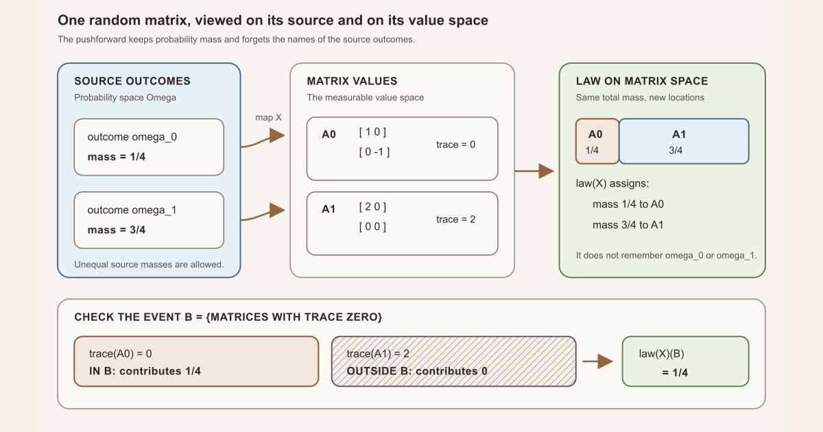
The probability distribution, or law, of a random object assigns mass to measurable subsets of its value space. It is a probability measure, not the random object itself. The two names mean the same thing on this site.
Start with a two-atom matrix law
Let the outcome space be \(\Omega=\{\omega_0,\omega_1\}\), with
\[ \mathbb P\{\omega_0\}=\frac14, \qquad \mathbb P\{\omega_1\}=\frac34. \]Define two matrices
\[ A_0= \begin{bmatrix} 1&0\\ 0&-1 \end{bmatrix}, \qquad A_1= \begin{bmatrix} 2&0\\ 0&0 \end{bmatrix}, \]and define the random matrix \(X\) by
\[ X(\omega_0)=A_0, \qquad X(\omega_1)=A_1. \]Write \(\delta_A\) for a point mass concentrated at a matrix \(A\). Then
\[ \mathcal L(X) =\frac14\,\delta_{A_0}+\frac34\,\delta_{A_1}. \]This equation is a complete description of the law. For example, let \(B\) be the set of matrices with trace zero. The first matrix lies in \(B\) and the second does not, so
\[ \mathcal L(X)(B)=\frac14. \]The calculation can be checked directly from the source outcomes:
\[ X^{-1}(B)=\{\omega_0\}, \qquad \mathbb P\bigl(X^{-1}(B)\bigr)=\mathbb P\{\omega_0\}=\frac14. \]
The numbers are exact toy probabilities, not empirical measurements. Renaming \(\omega_0\) and \(\omega_1\) without changing their masses or matrix values does not change the law. Changing a mass does. If both outcomes mapped to \(A_0\), their masses would combine and the law would put total mass one at \(A_0\).
The general definition
Suppose \(\Omega\) is the set of outcomes, \(\mathcal F\) is the collection of events to which probabilities may be assigned, and \(\mathbb P\) is a probability measure on those events. Let \(S\) be a measurable value space . A measurable function
\[ X:(\Omega,\mathcal F)\longrightarrow S \]is a random element with values in \(S\). Its law, written \(\mathcal L(X)\) or \(X_*\mathbb P\), is the probability measure on \(S\) defined by
\[ \mathcal L(X)(B) {} = \mathbb P\bigl(X^{-1}(B)\bigr) {} = \mathbb P\{\omega\in\Omega:X(\omega)\in B\} \]for every measurable set \(B\subseteq S\). Here \(X^{-1}(B)\) is the event consisting of outcomes whose values land in \(B\). This construction is the pushforward measure \(X_*\mathbb P\).
Measurability is what ensures that the preimage \(X^{-1}(B)\) is an allowed event whenever \(B\) is a measurable target set. Without that condition, the displayed probability may not be defined.
What the law retains, and what it discards
The law retains every probability statement that depends only on the value of \(X\). It discards the names and internal structure of the outcomes in \(\Omega\).
| Layer | Question it answers | Two-matrix example |
|---|---|---|
| Outcome \(\omega\) | What happened in the underlying experiment? | Either \(\omega_0\) or \(\omega_1\) |
| Random object \(X\) | Which value does each outcome produce? | The map sending \(\omega_0\) to \(A_0\) and \(\omega_1\) to \(A_1\) |
| Realization \(X(\omega)\) | Which value appeared for this outcome? | One ordinary matrix, \(A_0\) or \(A_1\) |
| Law \(\mathcal L(X)\) | How is probability distributed across all values? | Mass \(1/4\) at \(A_0\) and \(3/4\) at \(A_1\) |
Two random objects can live on different probability spaces and still have the same law. If \(X\) and \(Y\) both take values in the same measurable space \(S\), then
\[ X\mathrel{\overset{d}{=}}Y \quad\Longleftrightarrow\quad \mathcal L(X)=\mathcal L(Y). \]The notation \(X\mathrel{\overset{d}{=}}Y\) is read “equal in distribution.” It does not say that \(X=Y\) pointwise, or even that \(X\) and \(Y\) share a sample space.
A law is not automatically a density
The law is the probability measure itself. A probability mass function, a density, or a cumulative distribution function is a way to describe certain laws when additional structure is available.
| Object | What it records | Does every law have one? | In the example |
|---|---|---|---|
| Law \(\mathcal L(X)\) | A probability for every measurable target set | Yes, once \(X\) is measurable | \(\frac14\delta_{A_0}+\frac34\delta_{A_1}\) |
| Probability mass function (PMF) \(p(a)=\mathbb P\{X=a\}\) | Mass at each value of a discrete random object | No; it is a discrete representation | \(p(A_0)=1/4\), \(p(A_1)=3/4\) |
| Density \(f\) relative to a reference measure \(\lambda\) | \(\mathcal L(X)(B)=\int_B f\,d\lambda\) | No; some laws have atoms and no density relative to Lebesgue measure | The two-atom law has no ordinary Lebesgue density on matrix coordinates |
| Cumulative distribution function (CDF) \(F(t)=\mathbb P\{X\le t\}\) | Probabilities of lower half-lines for a real-valued object | Only for an ordered real-valued setting | Not the natural description of a matrix-valued object |
The finite law does have a PMF on its two-point support. Equivalently, that PMF can be viewed as a density relative to counting measure, but this does not turn it into a density relative to every other reference measure. Always name the reference measure when saying “density.”
The distinction between a random object and its law is equally important. The random object \(X\) is a function of an outcome. Its law \(\mathcal L(X)\) is a measure on the value space. Knowing the law does not reconstruct the fibers of \(X\), its exact set-theoretic range on null sets, or which outcome was mapped to which value.
From a matrix law to an observable law
A scalar quantity computed from a matrix is an observable. If \(T\) is another measurable space and \(f:S\to T\) is measurable, then \(f(X)\) is a random element in \(T\), and
\[ \mathcal L(f(X))=f_*\mathcal L(X). \]For the matrix \(X\) above, the trace observable takes values \(0\) and \(2\) with probabilities \(1/4\) and \(3/4\). Its law is therefore
\[ \mathcal L(\operatorname{tr}X) =\frac14\,\delta_0+\frac34\,\delta_2. \]This passage from a matrix law to an observable law is how eigenvalues, traces, norms, and other matrix statistics become ordinary probability distributions. Measurability of the observable is a real proof obligation. A formula alone does not automatically define a random variable.
In Lean
Mathlib writes a pushforward as Measure.map. The project wraps that
construction in RandomMatrix.law while keeping the measurability
proof visible.
RandomMatrix.law X hX μ s = μ (X ⁻¹' s)RandomMatrix.law X hX μis the target-space measureMeasure.map X μ.Xis the matrix-valued function, andhX : Measurable Xis the proof that preimages of measurable target sets are measurable source events.μis the source measure. The same map can have different laws under different source measures.sis a target set, with a separate hypothesishs : MeasurableSet sin the theorem.X ⁻¹’ sis Lean’s notation for the set-theoretic preimage ofsunderX. It is the Lean counterpart of \(X^{-1}(s)\).
Small standalone tutorial: push the two quarter-weights forward
The exact matrices \(A_0\) and \(A_1\) from the worked example can be treated
as two symbolic values while Lean checks the finite probability ledger. The
source weights are stored in quarters, so \(1\) means \(1/4\) and \(3\) means
\(3/4\). Create /tmp/TwoMatrixLaw.lean with these contents:
import Std

namespace TwoMatrixLaw

inductive Outcome
  | omega0
  | omega1
  deriving DecidableEq, Repr

inductive MatrixValue
  | a0
  | a1
  deriving DecidableEq, Repr

def outcomes : List Outcome :=
  [.omega0, .omega1]

def sourceMassQuarters : Outcome → Nat
  | .omega0 => 1
  | .omega1 => 3

def randomMatrix : Outcome → MatrixValue
  | .omega0 => .a0
  | .omega1 => .a1

def traceZero : MatrixValue → Bool
  | .a0 => true
  | .a1 => false

def lawMassQuarters (targetEvent : MatrixValue → Bool) : Nat :=
  outcomes.foldl
    (fun total omega =>
      if targetEvent (randomMatrix omega) then
        total + sourceMassQuarters omega
      else
        total)
    0

#eval lawMassQuarters traceZero
#eval lawMassQuarters (fun _ => true)

example : lawMassQuarters traceZero = 1 := by decide
example : lawMassQuarters (fun _ => true) = 4 := by decide

end TwoMatrixLaw
From any directory on a normal macOS or Linux machine with the pinned compiler, type exactly:
source "$HOME/.elan/env"
elan run leanprover/lean4:v4.32.0 lean /tmp/TwoMatrixLaw.lean
This exact worksheet was executed successfully with Lean 4.32.0 while repairing this page. It printed:
1
4
The first line says the trace-zero target event receives one quarter of the
mass because only \(\omega_0\) maps to \(A_0\). The second confirms that the
whole target space receives all four quarters. This Std-only
tutorial checks the finite pushforward arithmetic. It intentionally leaves
matrix algebra, measurability, and Measure.map to the exact
project interface below.
Exact project and Mathlib interface
The following is an exact excerpt from the checked project module. The definition exposes the pushforward, and the theorem reduces its value on a measurable set to the preimage calculation used in the example.
noncomputable def law (X : RandomMatrix Ω ι ι ℂ) (_hX : Measurable X)
    (μ : Measure Ω) : Measure (Matrix ι ι ℂ) :=
  Measure.map X μ

theorem law_apply (X : RandomMatrix Ω ι ι ℂ) (hX : Measurable X)
    (μ : Measure Ω) {s : Set (Matrix ι ι ℂ)} (hs : MeasurableSet s) :
    law X hX μ s = μ (X ⁻¹' s) := by
  exact Measure.map_apply hX hs
The same module proves law_comp for measurable matrix
endomorphisms, law_isProbabilityMeasure when the source measure
is a probability measure, and law_dirac for a point-mass source.
The bundled HermitianRandomMatrix.law reuses the measurability
field already stored in a Hermitian random matrix.
The source measure remains an explicit argument rather than a field of
RandomMatrix. That makes the dependence of the law on the chosen
measure visible. Mathlib’s underlying Measure.map is totalized to
the zero measure when its map is not almost-everywhere measurable. The
project’s RandomMatrix.law requires measurability and does not use
that fallback as a hidden probabilistic assumption.
The authoritative source is
formalization/NonlinearDynamics/Random/RandomMatrices/Laws.lean.
A learner can put these lines in a temporary scratch file inside a clone with
the repository’s pinned dependencies installed:
import NonlinearDynamics.Random.RandomMatrices.Laws

#print NonlinearDynamics.Random.RandomMatrix.law
#check NonlinearDynamics.Random.RandomMatrix.law_apply
#print shows the definition behind the name. #check
asks Lean to elaborate the following identifier and report its type; it does
not create a new theorem. The command below checks the authoritative project
module itself.
cd formalization
lake env lean -DwarningAsError=true NonlinearDynamics/Random/RandomMatrices/Laws.lean
Resource note: this exact file uses the repository's
pinned Lean and Mathlib dependencies. Initial project setup can require
substantial disk space and build time. For a lightweight first step on
macOS or Linux, use the page's standalone Lean-core or Std
tutorial.
Distinctions that prevent common mistakes
| Do not confuse | With | Why the difference matters |
|---|---|---|
| A random matrix \(X\) | Its law \(\mathcal L(X)\) | One is a function; the other is a measure on matrix space |
| Equal laws | Pointwise equality | Different functions, even on different spaces, can have the same law |
| A marginal entry law | The joint matrix law | Marginals do not record dependence among entries |
| A law | A density, PMF, or CDF | The law is a measure; the other objects are representations available in particular settings |
| Full law mass on Hermitian matrices | unitary invariance | The first makes the non-Hermitian locus null; the second is a symmetry of the law. Neither phrase alone identifies a particular sample map’s pointwise range |
| Measurability | Integrability | A measurable observable need not have a finite expectation |
Knowing every one-entry marginal law is generally not enough to recover the matrix law. Correlations between entries are part of the joint law. This is especially important for a Hermitian matrix , whose reflected off-diagonal entries are linked by complex conjugation.
Where to continue
The random matrix page separates a map from one of its realized values. The pushforward measure page studies the construction \(X_*\mathbb P\) itself. The measurable space page explains why measurability must come before a law. For the full learning path, continue to Random Matrices: From Outcomes to Spectra. The first complete named ensemble construction is developed in Finite GUE from Independent Gaussian Coordinates.
References
Olav Kallenberg. Foundations of Modern Probability, third edition, Springer, 2021. This is a standard source for random elements, their distributions, and measurable mappings.
Mathlib contributors.
Pushforward of a measure,
Mathlib 4 documentation. This official implementation reference documents
Measure.map, map_apply, and the non-measurable
fallback described above.
Greg W. Anderson, Alice Guionnet, and Ofer Zeitouni. An Introduction to Random Matrices, Cambridge University Press, 2010. This develops matrix ensembles as probability laws and tracks the additional symmetry and normalization assumptions needed for the classical models.