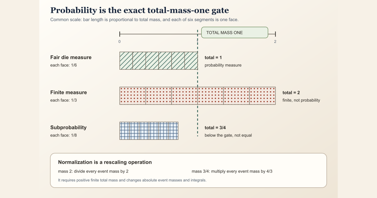
A probability measure is a measure whose total mass is exactly one. If \(\Omega\) is the entire outcome space and \(\mathbb P\) is the measure, the defining normalization is
\[ \mathbb P(\Omega)=1. \]Nonnegativity and countable additivity come from being a measure. Total mass one is the extra condition that turns mass into probability.
Start with one fair die
Let
\[ \Omega=\{1,2,3,4,5,6\} \]be the possible outcomes of a fair six-sided die. Assign every face mass \(1/6\):
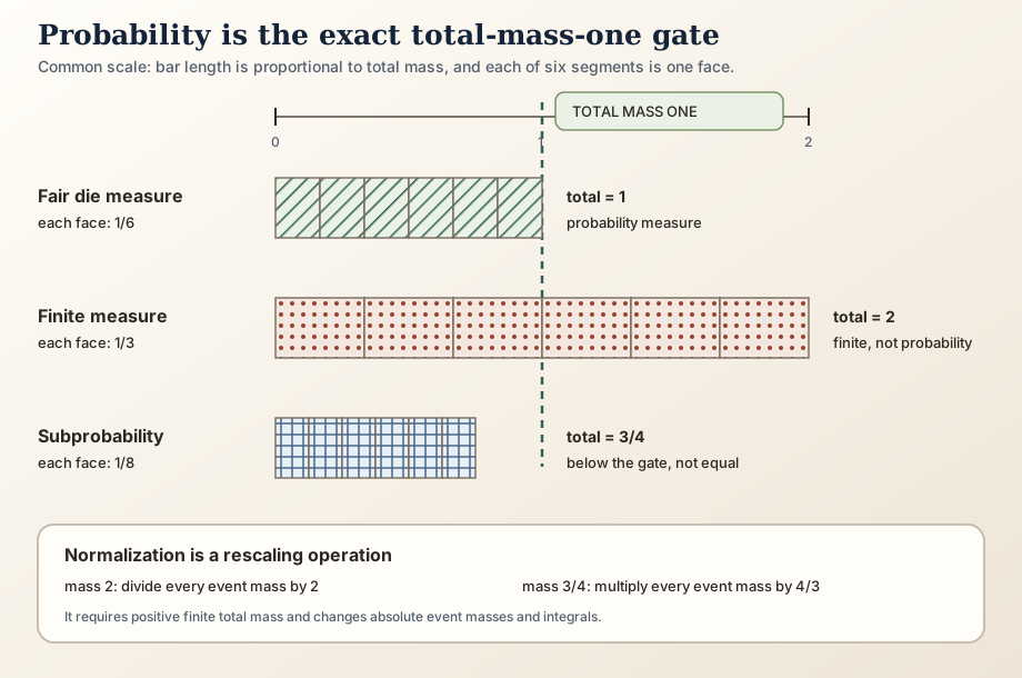
\[ \mathbb P\{k\}=\frac16 \qquad\text{for each }k\in\Omega. \]The six singleton events are disjoint and their union is the whole space, so finite additivity gives
\[ \mathbb P(\Omega) =\sum_{k=1}^{6}\mathbb P\{k\} =6\cdot\frac16 =1. \]Thus \(\mathbb P\) is a probability measure. For the event
\[ E=\{2,4,6\} \quad\text{(the roll is even)}, \]we calculate
\[ \mathbb P(E)=3\cdot\frac16=\frac12. \]The number \(1/2\) is not an extra label attached to \(E\). It is the measure of that set under this particular total-mass-one measure.
Two nearby measures that are not probabilities
Keep the same six-point space but change the mass per face.
First define \(\nu\{k\}=1/3\). Its total mass is
\[ \nu(\Omega)=6\cdot\frac13=2. \]This is a finite measure because its total mass is finite. It is not a probability measure because the total is two rather than one. The even event has \(\nu(E)=3\cdot(1/3)=1\); that value does not mean the event is certain, because certainty language is licensed only after total mass is one.
Next define \(\rho\{k\}=1/8\). Its total mass is
\[ \rho(\Omega)=6\cdot\frac18=\frac34. \]This is a subprobability measure: its total mass is at most one, but here it is strictly below one. The even event has
\[ \rho(E)=3\cdot\frac18=\frac38. \]Neither finiteness nor the upper bound \(\rho(\Omega)\le1\) is the defining probability condition. The gate is exact equality with one.
The exact definition
Let \((\Omega,\mathcal F)\) be a measurable space. A probability measure is a measure
\[ \mathbb P:\mathcal F\longrightarrow[0,\infty] \]with the following properties:
- \(\mathbb P(A)\ge0\) for every measurable event \(A\);
- \(\mathbb P\) is countably additive on pairwise disjoint events; and
- \(\mathbb P(\Omega)=1\).
The first two are the ordinary measure axioms. The third is the probability normalization. Monotonicity then gives
\[ 0\le\mathbb P(A)\le1 \]for every event \(A\), because \(A\subseteq\Omega\) and measures are monotone.
For a measurable event \(A\), its complement satisfies
\[ \mathbb P(A^{\mathsf c})=1-\mathbb P(A). \]That familiar probability formula is the ordinary measure identity \(\mathbb P(A)+\mathbb P(A^{\mathsf c})=\mathbb P(\Omega)\) with total mass one substituted at the final step.
Normalizing a finite measure
Suppose \(\nu\) is a finite measure with strictly positive total mass:
\[ 0\lt\nu(\Omega)\lt\infty. \]Then the rescaled measure
\[ \widehat\nu(A)=\frac{\nu(A)}{\nu(\Omega)} \]is a probability measure, because
\[ \widehat\nu(\Omega) =\frac{\nu(\Omega)}{\nu(\Omega)} =1. \]For the mass-two die measure, normalization divides every event mass by two:
\[ \widehat\nu\{k\}=\frac16, \qquad \widehat\nu(E)=\frac12. \]For the mass-three-quarters subprobability, normalization multiplies every event mass by \(4/3\):
\[ \widehat\rho\{k\}=\frac16, \qquad \widehat\rho(E)=\frac12. \]The two normalized measures happen to become the same fair-die law because both original examples gave equal weight to every face.
Why normalization is not always harmless
Rescaling preserves which sets have mass zero and preserves ratios of positive finite event masses. It does not preserve the original absolute scale. In the mass-two model, the even set changes from mass one to probability one half. An integral \(\int f\,d\nu\) is divided by the same total mass, so a physical quantity such as particle intensity, spatial density, or expected count can change meaning.
Normalization also requires a positive finite denominator:
- the zero measure has \(\nu(\Omega)=0\), so division by the total cannot produce a probability measure;
- an infinite measure has \(\nu(\Omega)=\infty\), so constant rescaling does not turn it into a total-mass-one measure; and
- a measure chosen for its absolute units may be intentionally unnormalized.
Therefore “normalize the measure” is a mathematical operation with preconditions and semantic consequences, not a free change of notation.
Probability measure, law, and density are different layers
A probability measure can be specified directly, as with the fair die. It can also arise as the probability law of a random object, obtained by pushing a source probability measure onto a value space.
A density is only one possible representation of a measure relative to a chosen reference measure. The fair die has a probability mass function. A Dirac probability measure concentrates all mass at one point. A continuous law may have a density, but not every probability measure does. “Probability measure” names the measure itself, not a formula used to describe it.
A null set is also measure-relative. Rescaling a positive finite measure to a probability measure preserves its null sets, but changing to an unrelated probability measure can change which sets are null.
In Lean: total mass one is a typeclass gate
Mathlib represents the normalization as a proposition-valued typeclass. In a theorem, square brackets ask Lean to find or receive the probability-measure certificate automatically.
example [IsProbabilityMeasure μ] : μ univ = 1 := measure_univμhas typeMeasure Ωfor some measurable outcome typeΩ.[IsProbabilityMeasure μ]is an implicit typeclass assumption. Its data is a proof of the mass-one equation.univ : Set Ωis the set of all outcomes, the Lean counterpart of \(\Omega\) in the displayed formula.μ univapplies the measure to the whole set.measure_univis the theorem exported from the typeclass. Under the square-bracket assumption, it supplies the proof ofμ univ = 1.- The numeral
1is interpreted in the measure’s extended nonnegative-real codomain.
Small standalone tutorial: test the total-mass gate
Put all three six-face examples over the common denominator \(24\). A fair
face has mass \(4/24=1/6\), a face in the mass-two model has
\(8/24=1/3\), and a face in the subprobability model has
\(3/24=1/8\). Total mass one is therefore exactly total numerator \(24\).
Create /tmp/ProbabilityMassGate.lean with these contents:
import Std

namespace ProbabilityMassGate

def totalTwentyFourths (perFaceTwentyFourths : Nat) : Nat :=
  6 * perFaceTwentyFourths

def hasTotalMassOne (perFaceTwentyFourths : Nat) : Bool :=
  totalTwentyFourths perFaceTwentyFourths == 24

#eval [
  totalTwentyFourths 4,
  totalTwentyFourths 8,
  totalTwentyFourths 3
]
#eval [
  hasTotalMassOne 4,
  hasTotalMassOne 8,
  hasTotalMassOne 3
]

example : totalTwentyFourths 4 = 24 := by decide
example : totalTwentyFourths 8 = 48 := by decide
example : totalTwentyFourths 3 = 18 := by decide
example : hasTotalMassOne 4 = true := by decide
example : hasTotalMassOne 8 = false := by decide
example : hasTotalMassOne 3 = false := by decide

end ProbabilityMassGate
From any directory on a normal macOS or Linux machine with the pinned compiler, type exactly:
source "$HOME/.elan/env"
elan run leanprover/lean4:v4.32.0 lean /tmp/ProbabilityMassGate.lean
This exact worksheet was executed successfully with Lean 4.32.0 while repairing this page. It printed:
[24, 48, 18]
[true, false, false]
Dividing the first row by \(24\) recovers the exact totals \(1\), \(2\), and
\(3/4\). Only the first Boolean is true because only that total equals one.
This bounded arithmetic model imports only Std. It illustrates
the normalization gate; it does not construct Mathlib measures.
Exact project and Mathlib interface
The project uses the typeclass as a semantic gate, not as a hidden
renormalization operation. The following definition and theorem are exact
excerpts from ProbabilityErgodicBase.lean:
def finiteHorizonLogPlusExpectation [IsProbabilityMeasure μ]
    (C : DiscreteMatrixCocycle (ι := ι) μ)
    (_hC : C.HasIntegrableGeneratorLogPlus) (k : ℕ) : ℝ :=
  ∫ ω, C.logPlusNormObservable k ω ∂μ

@[simp] theorem finiteHorizonLogPlusExpectation_eq_integratedLogPlusNorm
    [IsProbabilityMeasure μ]
    {C : DiscreteMatrixCocycle (ι := ι) μ}
    (hC : C.HasIntegrableGeneratorLogPlus) (k : ℕ) :
    C.finiteHorizonLogPlusExpectation hC k = C.integratedLogPlusNorm k := by
  rfl
The definition does not divide by \(\mu(\Omega)\). The square-bracket premise
already certifies that \(\mu(\Omega)=1\), so the raw integral is correctly
identified as an expectation. The equality proof is rfl, meaning
both sides reduce to the same expression by definition. Probability here
changes which terminology and theorems are licensed; it does not silently
change the measure supplied by the caller.
The same module uses [IsProbabilityMeasure μ] in its checked
zero-or-one theorem for a measurable invariant event. The outcomes \(0\) and
\(1\) are probability values only because the total-mass-one gate is visible.
The authoritative checked source is
formalization/NonlinearDynamics/Random/RandomCocycles/ProbabilityErgodicBase.lean.
A human can type the following worksheet in a scratch buffer inside a clone
with the repository’s pinned dependencies installed:
import NonlinearDynamics.Random.RandomCocycles.ProbabilityErgodicBase

open MeasureTheory Set

#check IsProbabilityMeasure
#check measure_univ
#check isProbabilityMeasure_iff
#check NonlinearDynamics.Random.RandomCocycles.DiscreteMatrixCocycle.finiteHorizonLogPlusExpectation
#check NonlinearDynamics.Random.RandomCocycles.DiscreteMatrixCocycle.ergodicBase_invariantEvent_prob_eq_zero_or_one

example {Ω : Type*} [MeasurableSpace Ω] (μ : Measure Ω)
    [IsProbabilityMeasure μ] : μ univ = 1 :=
  measure_univ
The first three #check commands expose Mathlib’s class and its
defining equation. The next two inspect real project declarations whose
probability language is guarded by that class. The final example
asks Lean to recover the mass-one equation from the typeclass assumption. The
full-project command below checks the complete project module containing the exact
excerpt.
cd formalization
lake env lean -DwarningAsError=true NonlinearDynamics/Random/RandomCocycles/ProbabilityErgodicBase.lean
Resource note: this exact file uses the repository's
pinned Lean and Mathlib dependencies. Initial project setup can require
substantial disk space and build time. For a lightweight first step on
macOS or Linux, use the page's standalone Lean-core or Std
tutorial.
Boundaries that prevent common mistakes
| Tempting shortcut | Correct statement |
|---|---|
| “Every finite measure is a probability measure.” | A finite measure only has finite total mass; a probability measure has total mass exactly one. |
| “A subprobability is already a probability.” | A subprobability may have total mass below one. Equality with one is required. |
| “Event mass one always means certainty.” | That language assumes the whole space also has mass one. Under the mass-two measure, a proper event can have mass one. |
| “Normalization changes nothing.” | It preserves relative mass and null sets under positive finite scaling, but changes absolute event masses and integrals. |
| “Every measure can be normalized.” | Constant normalization needs strictly positive finite total mass. |
| “Probability measure means density.” | A density is an optional representation relative to another measure. |
Where to continue
The measure entry develops nonnegativity, countable additivity, and total mass without assuming normalization. The event entry teaches the measurable sets to which probabilities are assigned. The probability distribution (law) entry shows how a measurable random object transports a probability measure to its value space. The null set entry explains zero-mass exceptions and why they need not be empty.
For the project use of this gate, continue to Probability Normalization and Ergodic Rigidity Before Kingman. It separates finite-horizon integrability, probability normalization, measure preservation, and ergodicity before any samplewise convergence claim.
References
Mathlib contributors.
Probability-measure typeclasses,
Mathlib 4 documentation. This official source defines
IsProbabilityMeasure by μ univ = 1 and derives the
standard probability bounds and complement identities.
Olav Kallenberg. Foundations of Modern Probability, third edition, Springer, 2021. This is a standard reference for probability measures, distributions, and normalization.
Project source. ProbabilityErgodicBase.lean contains the checked expectation and invariant-event interfaces used in the Lean section.