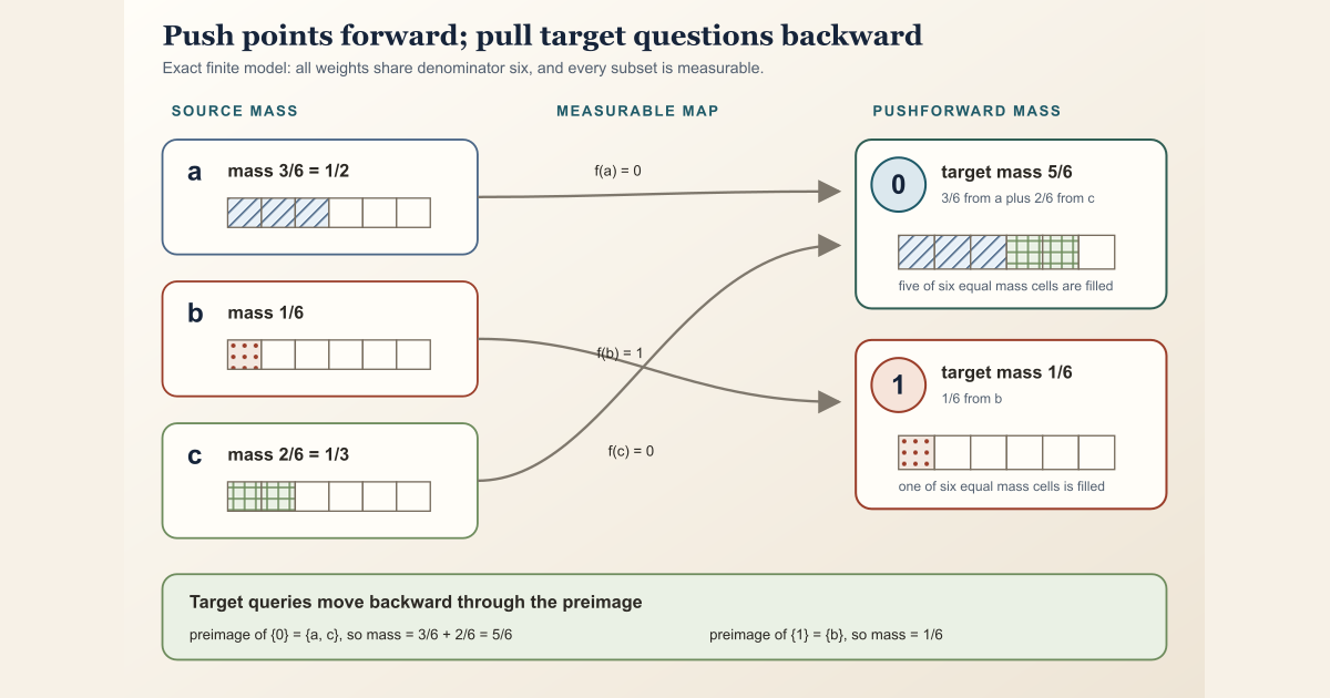
A pushforward measure transports mass from one measurable space to another through a function. Points move forward, but the mass of a target set is computed from all source points that map into it.
Let \((S,\mathcal A)\) and \((T,\mathcal B)\) be measurable spaces. Here \(S\) and \(T\) are sets, while \(\mathcal A\) and \(\mathcal B\) are their collections of measurable subsets. Let \(\mu\) be a measure on \(S\), and let
\[ f:S\longrightarrow T \]be measurable. This means that for every measurable target set \(B\in\mathcal B\), its preimage \(f^{-1}(B)\) belongs to the source collection \(\mathcal A\). The pushforward of \(\mu\) by \(f\) is the measure \(f_*\mu\) on \(T\) defined by
\[ (f_*\mu)(B)=\mu\bigl(f^{-1}(B)\bigr) \]for every measurable set \(B\in\mathcal B\). Other common notations are \(\mu\circ f^{-1}\) and \(f_\#\mu\).
The inverse image is essential. Measures are evaluated on sets, while \(f\) sends points forward. To learn how much source mass arrives in \(B\), we collect the source points that land there and measure that collection with \(\mu\). Measurability is exactly the guarantee that this collected source set is an event to which the source measure applies in the ordinary measure-space sense.
The transport picture
| Stage | Object | Operation |
|---|---|---|
| Source | A measure \(\mu\) on \(S\) | Start with mass assigned to source sets |
| Map | A measurable function \(f:S\to T\) | Send each source point to one target point |
| Target | The measure \(f_*\mu\) on \(T\) | Assign each target set the mass of its preimage |
The two directions must be distinguished: \(f\) maps source points to target points, while \(f^{-1}\) maps target sets to source sets. The next example makes both directions explicit.
A finite example with collisions
Take the source set \(S=\{a,b,c\}\) and assign masses
\[ \mu\{a\}=\frac12, \qquad \mu\{b\}=\frac16, \qquad \mu\{c\}=\frac13. \]Let the target set be \(T=\{0,1\}\), and define
\[ f(a)=0, \qquad f(b)=1, \qquad f(c)=0. \]Give both finite sets the measurable structure in which every subset is measurable. Then \(f\) is automatically measurable: the preimage of any target subset is a source subset.
Two source points collide at the target value \(0\). Therefore
\[ \begin{aligned} (f_*\mu)\{0\} &=\mu\bigl(f^{-1}\{0\}\bigr) =\mu\{a,c\} =\frac12+\frac13 =\frac56,\\ (f_*\mu)\{1\} &=\mu\bigl(f^{-1}\{1\}\bigr) =\mu\{b\} =\frac16. \end{aligned} \]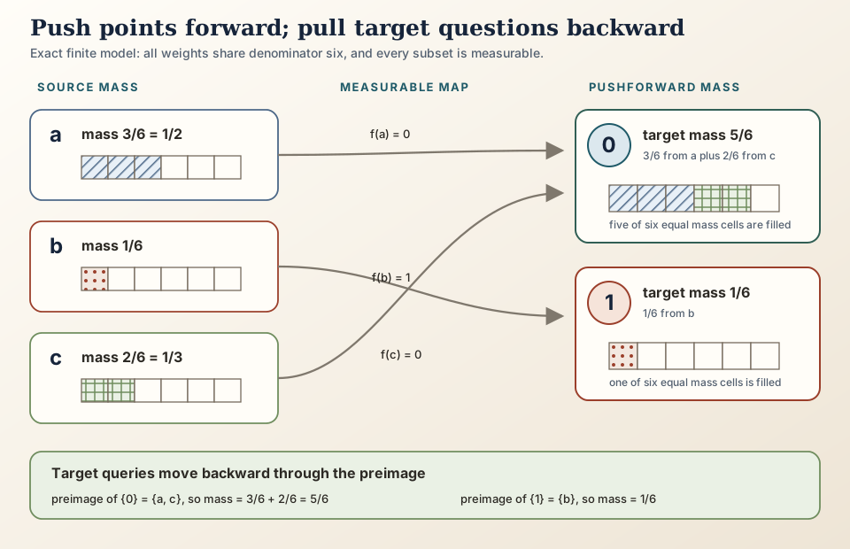
The total mass remains one. The pushforward combines mass when several source points have the same image. It does not retain whether \(a\) or \(c\) produced the target value \(0\) if all we retain is the target value. The colored and patterned encoding in the teaching figure retains that provenance only so the arithmetic can be inspected; the pushforward measure itself stores the total \(5/6\), not a source label on each part.
Probability laws are pushforwards
Let \(X:\Omega\to S\) be a random element on a probability space \((\Omega,\mathcal F,\mathbb P)\). Its probability law is exactly
\[ \mathcal L(X)=X_*\mathbb P. \]Thus a law is not an unrelated object added after the random variable. It is the source probability measure transported through that random variable.
For a random matrix \(X:\Omega\to\mathbb C^{n\times n}\), the same formula produces a measure on matrix space:
\[ \mathcal L(X)=X_*\mathbb P. \]The source outcomes disappear from the target description. What remains is the probability assigned to each measurable region of matrix space.
A matrix observable as a second pushforward
Suppose \(\nu\) is a measure on square complex matrices, and let
\[ \tau(H)=\operatorname{tr}(H) \]be the matrix trace . When \(\tau\) is measurable, its pushforward \(\tau_*\nu\) is the distribution of the trace.
If \(\nu=\mathcal L(X)=X_*\mathbb P\), then the composition rule gives
\[ \mathcal L(\operatorname{tr}X) =\tau_*\bigl(X_*\mathbb P\bigr) =(\tau\circ X)_*\mathbb P. \]This identity says that the two routes agree:
- first form the matrix law and then push it through trace; or
- first compute trace sample by sample and then take the scalar law.
The same pattern applies to \(H\mapsto\operatorname{tr}(H^k)\), eigenvalue maps once their measurability is proved, matrix norms, and other observables.
Three structural identities
Pushforward has a small algebra that is worth remembering.
Identity map
For the identity function \(\operatorname{id}_S\),
\[ (\operatorname{id}_S)_*\mu=\mu. \]Composition
If \(R\) is a third measurable space, and \(f:S\to T\) and \(g:T\to R\) are measurable, then
\[ (g\circ f)_*\mu=g_*\bigl(f_*\mu\bigr). \]Total mass
Because \(f^{-1}(T)=S\),
\[ (f_*\mu)(T)=\mu(S). \]In particular, the pushforward of a probability measure by a measurable function is again a probability measure.
Integrating after transport
Pushforward also converts an integral over the target into an integral over the source. Under the standard measurability hypotheses, and for a nonnegative measurable function \(\varphi:T\to[0,\infty]\),
\[ \int_T \varphi(t)\,(f_*\mu)(dt) =\int_S \varphi(f(s))\,\mu(ds). \]For signed, real, or complex integrals, the corresponding integrability hypotheses are also required. This is the abstract form of “sample first, then average”: averaging a target observable under the transported law equals averaging its composition with the original random object.
In Lean: the preimage remains visible
Mathlib names pushforward Measure.map. The project uses that
construction to define the law of a measurable random matrix. Here is the core
statement in the three languages a reader must be able to translate between.
RandomMatrix.law X hX μ s = μ (X ⁻¹' s)RandomMatrix.law X hX μis the target-space measureMeasure.map X μ.Xsends source outcomes to matrix values.hX : Measurable Xproves that measurable target sets have measurable source preimages.μis the source measure. Changing it can change the pushforward even whenXstays fixed.sis the target set being queried. The checked theorem also takeshs : MeasurableSet s, which certifies that this query is measurable.X ⁻¹’ sis Lean’s set-preimage notation. Read it from right to left: start with target sets, then collect the source outcomes whoseX-values land there.- The equality says the target measure and source-preimage calculation return exactly the same extended nonnegative real number.
The following definition and theorem are an exact excerpt from the checked
project source. The measurability proof is an explicit argument of
law, even though the definition’s body is
Measure.map X μ.
noncomputable def law (X : RandomMatrix Ω ι ι ℂ) (_hX : Measurable X)
    (μ : Measure Ω) : Measure (Matrix ι ι ℂ) :=
  Measure.map X μ

theorem law_apply (X : RandomMatrix Ω ι ι ℂ) (hX : Measurable X)
    (μ : Measure Ω) {s : Set (Matrix ι ι ℂ)} (hs : MeasurableSet s) :
    law X hX μ s = μ (X ⁻¹' s) := by
  exact Measure.map_apply hX hs
The final proof line hands Mathlib the two gates its evaluation theorem needs:
hX proves the map measurable, and hs proves the target
set measurable. The conclusion then computes the pushforward by a preimage.
The same module proves composition without hiding either measurability proof:
theorem law_comp {X : RandomMatrix Ω ι ι ℂ} (hX : Measurable X)
    {f : Matrix ι ι ℂ → Matrix ι ι ℂ} (hf : Measurable f) (μ : Measure Ω) :
    law (f ∘ X) (hf.comp hX) μ = Measure.map f (law X hX μ) := by
  exact (Measure.map_map hf hX).symm
This is the Lean form of
\((f\circ X)_*\mu=f_*(X_*\mu)\). The proof needs
hf : Measurable f and hX : Measurable X separately;
the composition proof hf.comp hX certifies the left-hand map.
There is one implementation boundary to keep visible. Mathlib makes
Measure.map a total operation: it is the zero measure when the map
is not
almost-everywhere
measurable
with respect to the source measure. When the map is almost-everywhere
measurable, Mathlib chooses a measurable representative. This is useful library
engineering, but it is not permission to invent a probability law from an
unproved function. The project’s public RandomMatrix.law interface
asks for the stronger, simpler certificate Measurable X before it
uses Measure.map.
For the deterministic congruence map \(C_A(H)=AHA^*\), the module proves
measurable_congruence. Its checked
HermitianRandomMatrix.law_conjugateBy theorem says that the law of
\(A X A^*\) is the congruence pushforward of the law of \(X\). It identifies
the transformed law; it does not assert that the transformed law equals the
original one.
Move the three source masses locally
This bounded Std worksheet stores the source masses as integer
numbers of sixths. It computes preimages first and then adds the source mass
inside each one, exactly following the pushforward definition. Save it as
/tmp/PushforwardScratch.lean on a normal Mac or Linux computer:
import Std

namespace PushforwardScratch

def sourceAtoms : List String := ["a", "b", "c"]

def massSixths (source : String) : Nat :=
  if source == "a" then 3
  else if source == "b" then 1
  else 2

def target (source : String) : Nat :=
  if source == "b" then 1 else 0

def preimage (targetValue : Nat) : List String :=
  sourceAtoms.filter (fun source => target source == targetValue)

def pushMassSixths (targetValue : Nat) : Nat :=
  (preimage targetValue).foldl
    (fun total source => total + massSixths source) 0

#eval preimage 0
#eval preimage 1
#eval [pushMassSixths 0, pushMassSixths 1]
#eval pushMassSixths 0 + pushMassSixths 1

example : preimage 0 = ["a", "c"] := by decide
example : preimage 1 = ["b"] := by decide
example : pushMassSixths 0 = 5 := by decide
example : pushMassSixths 1 = 1 := by decide
example : pushMassSixths 0 + pushMassSixths 1 = 6 := by decide

end PushforwardScratch
Type these commands exactly:
source "$HOME/.elan/env"
elan run leanprover/lean4:v4.32.0 lean /tmp/PushforwardScratch.lean
This exact standalone worksheet was executed successfully with Lean 4.32.0. It printed:
["a", "c"]
["b"]
[5, 1]
6
The target masses are therefore \(5/6\) and \(1/6\), and the last line checks
that transport retains total mass one. This finite ledger does not construct
Mathlib’s Measure.map; it makes the preimage arithmetic visible
before the exact project interface below.
Full project check
The authoritative source is
formalization/NonlinearDynamics/Random/RandomMatrices/Laws.lean.
A human can type the following worksheet in a scratch buffer inside a clone with
the repository’s pinned dependencies installed:
import NonlinearDynamics.Random.RandomMatrices.Laws

#print NonlinearDynamics.Random.RandomMatrix.law
#check NonlinearDynamics.Random.RandomMatrix.law_apply
#check NonlinearDynamics.Random.RandomMatrix.law_comp
#check NonlinearDynamics.Random.HermitianRandomMatrix.law_conjugateBy
#print displays the checked definition behind a name.
#check asks Lean to elaborate a declaration and display its type;
it does not assume or prove an extra theorem. The full-project command below checks
the complete module containing the exact excerpts above.
cd formalization
lake env lean -DwarningAsError=true NonlinearDynamics/Random/RandomMatrices/Laws.lean
Resource note: this exact file uses the repository's
pinned Lean and Mathlib dependencies. Initial project setup can require
substantial disk space and build time. For a lightweight first step on
macOS or Linux, use the page's standalone Lean-core or Std
tutorial.
Distinctions and failure modes
| Tempting shortcut | What is wrong | Correct repair |
|---|---|---|
| “Push \(\mu\) forward by measuring \(f(A)\)” | Images of measurable sets are not the sets in the defining formula | Measure \(f^{-1}(B)\) for target sets \(B\) |
| “Every function gives the intended pushforward” | Measurability is needed for the preimage formula and probability interpretation | Prove measurable or almost-everywhere measurable first |
| “The inverse-image symbol means an inverse function” | A preimage exists even when the function is many-to-one or has no inverse function | Read the preimage as all source points that land in the target set |
| “Pushforward is a conditional distribution” | Conditioning changes mass using information; pushforward transports it through a function | Treat these as separate constructions |
| “The source outcome can be recovered from the pushforward” | Different source points can merge at one target point | Keep the original coupling when source-level information matters |
| “Equal observable pushforwards imply equal matrix laws” | One observable can discard most matrix information | Use a separating family of observables or prove equality of the full laws |
Where to continue
Read probability law for the special case of transporting a probability measure through a random object. Read measurable space for the source and target structures that make the preimage rule legal. Read random matrix and trace power for the source and observable in the project’s first examples. The chapter Random Matrices: From Outcomes to Spectra places the construction in the full probability-to-spectrum ascent. Finite GUE from Independent Gaussian Coordinates is the first project chapter to use this bridge on a complete Gaussian coordinate probability measure and obtain a named matrix law.
References
Mathlib contributors.
Pushforward of a measure,
Mathlib 4 documentation. This official implementation reference states the
definitions and main theorems map_apply and
map_map, including Mathlib’s behavior for maps that are not
almost-everywhere measurable.
Olav Kallenberg. Foundations of Modern Probability, third edition, Springer, 2021. This is a standard measure-theoretic reference for image measures, distributions of random elements, and integration under measurable mappings.
Mathlib contributors.
Measurable spaces and measurable functions,
Mathlib 4 documentation. This official source gives the measurability layer on
which Measure.map depends.