Random matrix

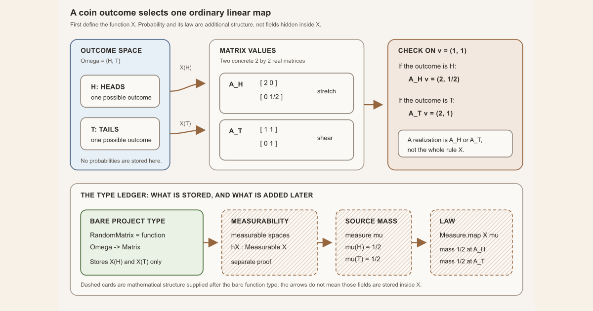
A random matrix is a rule that turns an outcome into an ordinary matrix. The rule is the whole object. A matrix seen in one run is only one of its realizations.

Start with a coin-selected linear map

Let the outcome space have two points:

\[ \Omega=\{H,T\}, \]

where \(H\) means heads and \(T\) means tails. Define two real matrices

\[ A_H= \begin{bmatrix} 2&0\\ 0&\frac12 \end{bmatrix}, \qquad A_T= \begin{bmatrix} 1&1\\ 0&1 \end{bmatrix}. \]

The first stretches the horizontal direction and compresses the vertical direction. The second is a shear. Define one matrix-valued function \(X\) by

\[ X(H)=A_H, \qquad X(T)=A_T. \]

This function is the random matrix. If we apply the realized matrix to \(v=(1,1)\), the two possible outputs are

\[ A_Hv=\left(2,\frac12\right), \qquad A_Tv=(2,1). \]

Every number in this example is directly checkable by matrix multiplication. Before assigning coin probabilities, \(X\) is already a perfectly good outcome-to-matrix function. It does not yet determine how likely either output is.

Heads maps to a diagonal stretch-compress matrix and tails maps to a shear matrix. On the vector one comma one, the two realized outputs are two comma one half and two comma one. A separate ledger shows that the project RandomMatrix type stores only the function, while measurability, a source measure, and the induced law are added later. — FigureFinding: the upper path is the concrete function \(X\): heads selects \(A_H\), tails selects \(A_T\), and one outcome produces one ordinary matrix realization. The vector check gives \(A_H(1,1)=(2,1/2)\) and \(A_T(1,1)=(2,1)\). The lower ledger separates what the project type stores from what later probability arguments supply. The solid green card is the bare function type. The dashed cards are a measurability proof, the fair source measure, and the resulting law with mass \(1/2\) at each matrix. Those dashed cards are not fields hidden inside \(X\).

Add probability without changing the function

Now equip \(\Omega\) with the fair-coin probability measure \(\mu\):

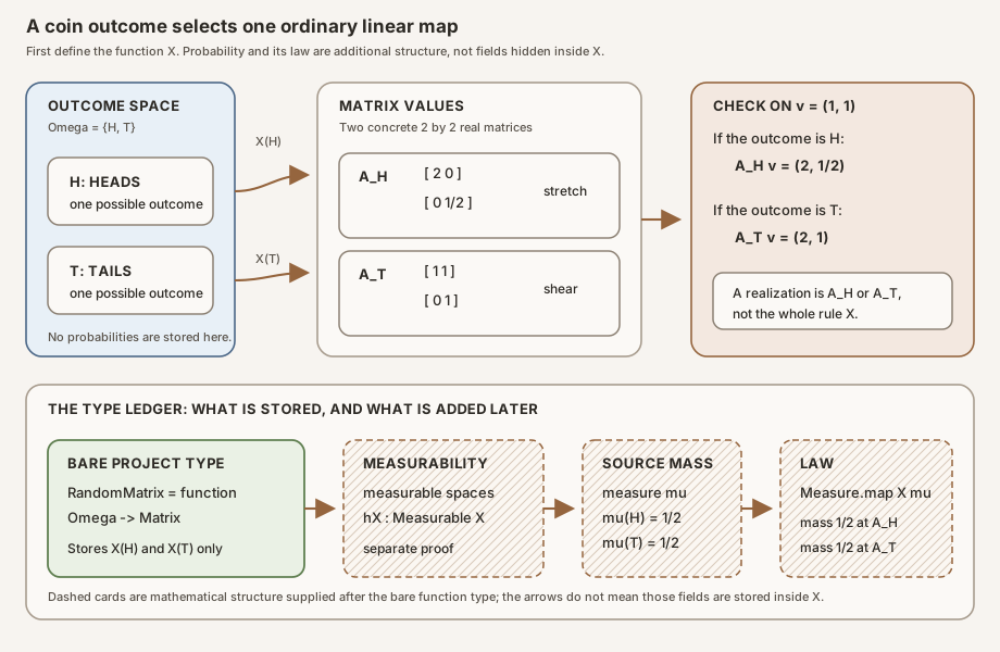
\[ \mu\{H\}=\mu\{T\}=\frac12. \]

The function \(X\) has not changed. What we have added is a measure on its source. Once measurability is available, the probability distribution (law) of \(X\) under \(\mu\) is

\[ \mathcal L_\mu(X) {} = \frac12\,\delta_{A_H}+\frac12\,\delta_{A_T}. \]

For example, let \(D\) be the set of diagonal matrices. Then \(A_H\in D\) and \(A_T\notin D\), so

\[ \mathcal L_\mu(X)(D)=\mu\bigl(X^{-1}(D)\bigr)=\mu\{H\}=\frac12. \]

If we keep exactly the same function \(X\) but instead choose \(\mu\{H\}=1/4\) and \(\mu\{T\}=3/4\), its law changes. This is why the project does not store a source measure inside its base RandomMatrix type.

Mathematical definition and project encoding

In probability theory, begin with a probability space \((\Omega,\mathcal F,\mathbb P)\). A random matrix over scalars \(\mathbb K\) is a measurable map

\[ X:\Omega\longrightarrow\mathbb K^{m\times n}, \]

usually with \(\mathbb K=\mathbb R\) or \(\mathbb C\). An outcome \(\omega\) selects the ordinary matrix \(X(\omega)\). Measurability says that allowed sets of matrices pull back to allowed events in \(\Omega\).

The project deliberately splits this definition into layers. Its base type is only the function. A measurable space , a proof that \(X\) is measurable, and a source measure are separate arguments or hypotheses. A law is then built as a pushforward measure .

Layer	What it answers	Coin example	Stored in the base type?
Outcome space \(\Omega\)	Which underlying cases are possible?	\(\{H,T\}\)	It appears as a type parameter
Matrix-valued map \(X\)	Which matrix belongs to each outcome?	\(H\mapsto A_H\), \(T\mapsto A_T\)	Yes; this is the function itself
Realization \(X(\omega)\)	Which ordinary matrix appeared now?	\(A_H\) or \(A_T\)	No; it is obtained by applying \(X\)
Measurability proof	Are preimages of target events allowed source events?	Automatic for this finite discrete model once the structures are chosen	No
Source measure \(\mu\)	How likely is each outcome?	\(1/2\) and \(1/2\)	No
Law \(\mathcal L_\mu(X)\)	How is probability spread over matrix values?	Half at each matrix	No

This separation keeps the same map reusable under different measures and in deterministic arguments that do not need probability.

Entries are scalar random variables

For a fixed row \(i\) and column \(j\), the coordinate map is

\[ \omega\longmapsto X(\omega)_{ij}. \]

If \(X\) is measurable for the entrywise matrix measurable space, each such coordinate is a measurable scalar random variable. Conversely, the checked project theorem says that if every coordinate is measurable, then \(X\) is measurable. This coordinate view is useful for constructing ensembles and stating moment assumptions. It does not imply that different coordinates are independent.

For example, a Hermitian matrix satisfies \(X(\omega)_{ji}=\overline{X(\omega)_{ij}}\) at every outcome when the Hermitian property is pointwise. The lower-triangular entries are then determined by the upper triangle, so declaring every coordinate independent would contradict the symmetry.

The Hermitian coordinate space makes the nonredundant primitive positions explicit: real diagonal values and complex strict-upper values are supplied, while the lower triangle is filled by conjugate reflection.

Boundaries and nonexamples

A single matrix \(A_H\) is not the random matrix \(X\). It is one possible value of \(X\).
A function can inhabit the project’s bare RandomMatrix alias before any measurable spaces, measurability proof, or probability measure have been supplied. At that stage it should not be credited with a law.
The word “random” does not mean that entries are independent or identically distributed. Those are additional properties of particular ensembles.
A law does not record which source outcome produced a matrix. The function \(X\) and its law are related, but they are different typed objects.

In Lean

The core translation is direct: the project name RandomMatrix abbreviates an ordinary function type.

One idea, three languages Read across, then read the syntax map

A human says

A project random matrix is a rule that accepts an outcome and returns one matrix. The base type alone contains no measurability proof and no probability measure.

On paper

\(X:\Omega\longrightarrow\mathbb K^{\iota\times\kappa}\).

In Lean

X : RandomMatrix Ω ι κ 𝕜

Syntax map

Ω is the type of outcomes.
ι and κ are the row-index and column-index types. They need not yet be finite.
𝕜 is the scalar type, such as ℝ or ℂ.
Matrix ι κ 𝕜 is the type of matrices with those row indices, column indices, and entries.
RandomMatrix Ω ι κ 𝕜 unfolds to Ω → Matrix ι κ 𝕜. The arrow → is the same outcome-to-value arrow shown on paper.
The absence of Measure and Measurable from this type is deliberate. They enter later as separate data and hypotheses.

Run the coin-selected map locally

The function-versus-probability distinction can be executed before importing Mathlib. This worksheet uses a four-field rational matrix and the exact vector \(v=(1,1)\) from the opening example. Save it as RandomMatrixScratch.lean in a scratch directory outside formalization/:

import Std

inductive Coin where
  | heads | tails
  deriving DecidableEq, Repr

structure Vec2 where
  x : Rat
  y : Rat
  deriving DecidableEq, Repr

structure Mat2 where
  a11 : Rat
  a12 : Rat
  a21 : Rat
  a22 : Rat
  deriving DecidableEq, Repr

def Mat2.act (A : Mat2) (v : Vec2) : Vec2 :=
  { x := A.a11 * v.x + A.a12 * v.y
    y := A.a21 * v.x + A.a22 * v.y }

def half : Rat :=
  1 / 2

def AH : Mat2 :=
  { a11 := 2, a12 := 0, a21 := 0, a22 := half }

def AT : Mat2 :=
  { a11 := 1, a12 := 1, a21 := 0, a22 := 1 }

def X : Coin → Mat2
  | .heads => AH
  | .tails => AT

def v : Vec2 :=
  { x := 1, y := 1 }

def headsResult : Vec2 :=
  { x := 2, y := half }

def tailsResult : Vec2 :=
  { x := 2, y := 1 }

#eval [decide (X Coin.heads = AH),
       decide (X Coin.tails = AT),
       decide ((X Coin.heads).act v = headsResult),
       decide ((X Coin.tails).act v = tailsResult)]

example : (X Coin.heads).act v = headsResult := by native_decide
example : (X Coin.tails).act v = tailsResult := by native_decide

Run it with exactly:

source "$HOME/.elan/env"
elan run leanprover/lean4:v4.32.0 lean RandomMatrixScratch.lean

This exact worksheet was executed successfully with Lean 4.32.0 and printed:

[true, true, true, true]

The first two booleans check the outcome-to-matrix function. The final two check \(A_Hv=(2,1/2)\) and \(A_Tv=(2,1)\). No probability appears in the file, which is the point: the sample map exists before a fair-coin measure is added. The two propositions use native_decide to normalize the exact rational arithmetic.

This bounded tutorial imports only Std and can run on a normal Mac or Linux machine. The general matrix alias and measurability theorem below are Mathlib-backed project interfaces and are full project checks.

Here is the exact base definition from the checked project module:

abbrev RandomMatrix
    (Ω : Type uΩ) (ι : Type uι) (κ : Type uκ) (𝕜 : Type u𝕜) :=
  Ω → Matrix ι κ 𝕜

Once measurable spaces have been supplied, the same module proves the exact coordinate criterion:

theorem measurable_iff_entries (X : RandomMatrix Ω ι κ 𝕜) :
    Measurable X ↔ ∀ i j, Measurable fun ω ↦ X ω i j := by
  rw [measurable_comap_iff]
  change Measurable (fun ω i j ↦ X ω i j) ↔ _
  simp only [measurable_pi_iff]

Read the right side as: for every row index i and column index j, the scalar function sending ω to the (i,j) entry of X ω is measurable. The symbol ↔ means the matrix-level and entry-level statements imply each other.

Try it in the repository NonlinearDynamics/Random/RandomMatrices/Basic.lean

The authoritative source is formalization/NonlinearDynamics/Random/RandomMatrices/Basic.lean. These are literal commands a learner can type in a temporary Lean file inside a clone with the repository’s pinned dependencies installed:

import NonlinearDynamics.Random.RandomMatrices.Basic

#print NonlinearDynamics.Random.RandomMatrix
#check NonlinearDynamics.Random.RandomMatrix.measurable_iff_entries
#check NonlinearDynamics.Random.RandomMatrix.measurable_entry

#print unfolds the abbreviation. Each #check asks Lean to elaborate the named theorem and show its type. The full-project command below checks the authoritative module rather than the temporary probe.

Full project check, from the repository root

cd formalization
lake env lean -DwarningAsError=true NonlinearDynamics/Random/RandomMatrices/Basic.lean

Resource note: this exact file uses the repository's pinned Lean and Mathlib dependencies. Initial project setup can require substantial disk space and build time. For a lightweight first step on macOS or Linux, use the page's standalone Lean-core or Std tutorial.

Where to continue

The probability distribution (law) page shows how a measurable random object and a source measure induce a measure on the value space. The almost-everywhere page separates pointwise properties from statements allowed to fail on a null set. For the deterministic assembly bridge, continue to Finite Hermitian Matrices from Coordinates.

Start with a coin-selected linear map

Add probability without changing the function

Mathematical definition and project encoding

Entries are scalar random variables

Boundaries and nonexamples

In Lean

Run the coin-selected map locally

Where to continue

Further reading