Random variable

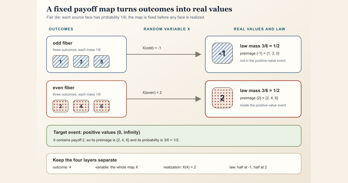
A real random variable is a measurable function that assigns a real number to every \(\omega\) in a sample space \(\Omega\). The function is fixed before an outcome is selected. What varies from one realization to another is the argument supplied to that function.

In symbols,

\[ X:\Omega\longrightarrow\mathbb R. \]

The word “variable” can be misleading at first. \(X\) is one entire function, not one unknown real number. Once an outcome \(\omega\) occurs, the ordinary number \(X(\omega)\) is the realized value.

Start with a fair-die payoff

Let

\[ \Omega=\{1,2,3,4,5,6\} \]

be the outcomes of a fair six-sided die, each with probability \(1/6\). Define a payoff random variable \(X:\Omega\to\mathbb R\) by

\[ X(k)= \begin{cases} -1,&k\text{ is odd},\\ 2,&k\text{ is even}. \end{cases} \]

Thus

\[ X(1)=X(3)=X(5)=-1, \qquad X(2)=X(4)=X(6)=2. \]

If the realized die outcome is \(\omega=4\), then the realization is the real number

\[ X(4)=2. \]

The outcome is \(4\); the random variable is the whole rule \(X\); and the realization is \(2\). Those are three different objects.

A fair die payoff map sends odd faces one, three, and five to minus one, and even faces two, four, and six to two. Each target value receives three sixths of the probability. The positive-value event pulls back to the even faces and has probability one half. — FigureFinding: the fixed map \(X\) sends three equally likely odd outcomes to payoff \(-1\) and three equally likely even outcomes to payoff \(2\). Therefore the induced law is \(\tfrac12\delta_{-1}+\tfrac12\delta_2\). The target event \((0,\infty)\) contains only the value \(2\), so its source preimage is \(\{2,4,6\}\) and its probability is \(3/6=1/2\). Patterns and direct labels distinguish the two fibers; the six source faces are exact possibilities, not six sampled rolls.

Pull a value-space event back to outcomes

Let the target event be the positive half-line

\[ B=(0,\infty)\subseteq\mathbb R. \]

To ask whether the payoff is positive, pull \(B\) back through \(X\):

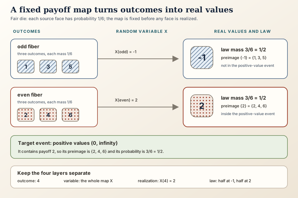
\[ \begin{aligned} X^{-1}(B) &=\{\omega\in\Omega:X(\omega)\in(0,\infty)\}\\ &=\{2,4,6\}. \end{aligned} \]

The preimage is an event in the outcome space. Its probability is

\[ \mathbb P\bigl(X^{-1}(B)\bigr) =\mathbb P\{2,4,6\} =\frac36 =\frac12. \]

This backward preimage is why measurability belongs in the definition of a random variable. Every measurable question about the reported real value must pull back to a measurable question about the underlying outcome.

Compute the induced distribution

The random variable takes only two values. Each value has three source outcomes, so

\[ \mathbb P\{X=-1\}=\frac12, \qquad \mathbb P\{X=2\}=\frac12. \]

Writing \(\delta_x\) for the point-mass probability measure at \(x\), the probability distribution (law) of \(X\) is

\[ \mathcal L(X) =X_*\mathbb P =\frac12\,\delta_{-1}+\frac12\,\delta_2. \]

The law is a probability measure on the value space \(\mathbb R\). It records the probability of every measurable set of values. For the positive half-line,

\[ \mathcal L(X)((0,\infty)) =\frac12 =\mathbb P\bigl(X^{-1}((0,\infty))\bigr). \]

The law does not retain which odd face produced \(-1\) or which even face produced \(2\). That information was merged by the many-to-one function \(X\).

Four layers that should not be conflated

Layer	Type of object	Die-payoff example	Question answered
Outcome \(\omega\)	one point of \(\Omega\)	\(4\)	What happened in this trial?
Random variable \(X\)	a measurable function \(\Omega\to\mathbb R\)	odd maps to \(-1\), even maps to \(2\)	How is every outcome converted to a number?
Realization \(X(\omega)\)	one real number	\(X(4)=2\)	What value did this outcome produce?
Law \(\mathcal L(X)\)	a probability measure on \(\mathbb R\)	half at \(-1\), half at \(2\)	What mass does each measurable target set receive?

Changing the realized outcome does not change the function or its law. Changing the payoff rule changes the random variable and usually changes its law. Changing the source probability measure can change the law even when the function stays fixed.

The exact definition

Let \((\Omega,\mathcal F,\mathbb P)\) be a probability space, and equip \(\mathbb R\) with its Borel measurable sets. A real random variable is a function

\[ X:\Omega\longrightarrow\mathbb R \]

such that for every Borel set \(B\subseteq\mathbb R\),

\[ X^{-1}(B)\in\mathcal F. \]

That condition says exactly that \(X\) is a measurable function . In the fair-die example, every source subset is measurable, so any real-valued function on the six outcomes is measurable. On a general outcome space, the proof can be a substantive obligation.

Some authors use “random variable” only for real-valued maps and “random element” for maps into a general measurable space. Others use “random variable” more broadly. This page uses the classical real-valued convention; the project’s random matrices are matrix-valued random elements.

“Random” names the probability-space role

The adjective does not assert a particular shape of distribution. A random variable need not be:

Gaussian;
independent of another random variable;
continuously distributed;
nonconstant;
unpredictable in an informal sense; or
generated by physical noise.

For example, the constant function \(X(\omega)=7\) is measurable and therefore is a random variable. Its law is the Dirac measure \(\delta_7\). It has no variation at all.

Independence is a relation among random variables or generated event collections under a specified measure. Gaussianity is a property of a law. Neither follows from the type \(X:\Omega\to\mathbb R\) or from measurability.

In Lean: the map and proof are separate inputs

Lean writes the sample map as an ordinary function and its measurability as a separate proposition.

One idea, three languages Read across, then read the syntax map

A human says

X assigns a real value to each outcome, and hX certifies that every measurable real-value event has a measurable source preimage.

On paper

\(X:\Omega\to\mathbb R\) with \(X^{-1}(B)\in\mathcal F\) for every Borel set \(B\).

In Lean

(X : Ω → ℝ) (hX : Measurable X)

Syntax map

X is the chosen name of the whole random variable.
Ω → ℝ is a function type. The arrow sends an outcome type to the real-number type.
Measurable X is a proposition, not another function. It states that X respects the installed measurable structures.
hX : gives a name to evidence for that proposition.
The standard measurable structure on ℝ is inferred from the target type. The source needs an instance [MeasurableSpace Ω].
The whole fragment is valid theorem-parameter syntax. Keeping both binders visible prevents a raw function from being treated as a random variable without its proof obligation.

Run the six-outcome payoff locally

The finite payoff, positive-event preimage, and two law masses can all be checked without importing a probability library. Save this as RandomVariableScratch.lean in a scratch directory outside formalization/:

import Std

def faces : List Nat :=
  [1, 2, 3, 4, 5, 6]

def payoff (face : Nat) : Int :=
  if face % 2 = 0 then 2 else -1

def positiveFaces : List Nat :=
  faces.filter (fun face => face % 2 == 0)

def countPayoff (value : Int) : Nat :=
  (faces.filter (fun face => payoff face == value)).length

#eval faces.map payoff
#eval positiveFaces
#eval (payoff 4, countPayoff (-1), countPayoff 2)

example : payoff 4 = 2 := by decide
example : positiveFaces = [2, 4, 6] := by decide
example : countPayoff (-1) = 3 := by decide
example : countPayoff 2 = 3 := by decide

Run it with the pinned compiler:

source "$HOME/.elan/env"
elan run leanprover/lean4:v4.32.0 lean RandomVariableScratch.lean

This exact worksheet was executed successfully with Lean 4.32.0 and printed:

[-1, 2, -1, 2, -1, 2]
[2, 4, 6]
(2, 3, 3)

The tuple says \(X(4)=2\), three faces map to \(-1\), and three map to \(2\). Because every face has mass \(1/6\), the last two counts give law masses \(3/6=1/2\). This tutorial checks only the exact finite ledger with Std, so it is bounded enough for a normal Mac or Linux machine. It does not define measures or prove measurability. The general Mathlib and project interfaces remain in the full project workflow below.

Given a source measure μ, Lean writes the induced value-space law as Measure.map X μ. For a measurable target set B, Measure.map_apply hX hB proves the same preimage equation used in the die calculation.

A real project interface: Gaussian coordinates

The project begins its Gaussian layer with real-valued functions. This is the exact checked definition of an explicitly parameterized Gaussian law:

def HasRealGaussianLaw (X : Ω → ℝ) (m : ℝ) (v : ℝ≥0) (P : Measure Ω) : Prop :=
  HasLaw X (gaussianReal m v) P

The function X : Ω → ℝ, mean m, nonnegative variance v, and source measure P remain separate inputs. Having this law supplies almost-everywhere measurability through Mathlib’s HasLaw; it does not silently upgrade the supplied representative to ordinary Measurable X.

For a family used as coordinate data, the project stores the stronger ordinary measurability and the additional probabilistic claims in separate fields:

structure IndependentRealGaussianFamily (X : ι → Ω → ℝ) (m : ι → ℝ)
    (v : ι → ℝ≥0) (P : Measure Ω) : Prop where
  measurable : ∀ i, Measurable (X i)
  hasLaw : ∀ i, HasRealGaussianLaw (X i) (m i) (v i) P
  independent : iIndepFun X P

This structure makes the distinctions executable. The measurable field says each coordinate is a random variable in the ordinary pointwise sense. The hasLaw field specifies each Gaussian distribution. The independent field is an additional joint property. None is inferred merely from the function type.

Try it in the repository NonlinearDynamics/Random/GaussianPrimitives.lean

The authoritative checked source is formalization/NonlinearDynamics/Random/GaussianPrimitives.lean. A human can type the following worksheet in a scratch buffer inside a clone with the repository’s pinned dependencies installed:

import NonlinearDynamics.Random.GaussianPrimitives

open MeasureTheory ProbabilityTheory
open NonlinearDynamics.Random

#check Measurable
#check HasRealGaussianLaw
#check IndependentRealGaussianFamily.measurable
#check IndependentRealGaussianFamily.hasLaw
#check IndependentRealGaussianFamily.independent
#check Measure.map_apply

example {Ω : Type*} [MeasurableSpace Ω] (c : ℝ) :
    Measurable (fun _ : Ω ↦ c) :=
  measurable_const

example {Ω : Type*} [MeasurableSpace Ω] (X : Ω → ℝ)
    (hX : Measurable X) (μ : Measure Ω) {B : Set ℝ}
    (hB : MeasurableSet B) :
    Measure.map X μ B = μ (X ⁻¹' B) :=
  Measure.map_apply hX hB

In the first example, Lean’s kernel checks a proof that a deterministic constant function is measurable. The second is the exact preimage computation behind a random variable’s law. The #check commands expose the project fields that keep measurability, Gaussian law, and independence separate. The full-project command below checks the complete project module containing the exact excerpts.

Full project check, from the repository root

cd formalization
lake env lean -DwarningAsError=true NonlinearDynamics/Random/GaussianPrimitives.lean

Resource note: this exact file uses the repository's pinned Lean and Mathlib dependencies. Initial project setup can require substantial disk space and build time. For a lightweight first step on macOS or Linux, use the page's standalone Lean-core or Std tutorial.

Boundaries that prevent common mistakes

Tempting shortcut	Correct statement
“The realized number is the random variable.”	The realized number is \(X(\omega)\); the random variable is the whole function \(X\).
“The law and variable are the same object.”	The variable is a sample map; its law is a pushed-forward probability measure.
“Any formula defines a random variable.”	The formula must define a function with the required measurability proof.
“Random means Gaussian.”	Gaussianity is one possible law-level property.
“Random means independent.”	Independence is an additional relation involving multiple variables or generated information.
“A constant is not random.”	A measurable constant function is a random variable with a Dirac law.

Where to continue

The event entry explains the source and target sets used in preimage questions. The measurable function entry develops the preimage gate directly, including a parity-only finite example. The probability distribution (law) entry separates a sample map from the probability measure it induces.

For the project’s first parameterized real-valued laws, continue to Gaussian Laws, Independence, and Normalization. It builds from real random variables to independent coordinate families and then toward finite random-matrix ensembles.

References

Olav Kallenberg. Foundations of Modern Probability, third edition, Springer, 2021. This is a standard reference for random variables, random elements, measurable mappings, and induced distributions.

Mathlib contributors. Laws of random variables, Mathlib 4 documentation. This official source documents the ProbabilityTheory.HasLaw interface imported by the checked project module.

Project source. GaussianPrimitives.lean contains the checked real Gaussian law and independent-coordinate interfaces used in the Lean section.