Trace-power observable

For a finite square matrix \(A\) and a nonnegative integer \(k\), the trace power

\[ \operatorname{tr}(A^k) \]

first multiplies the matrix by itself \(k\) times and then adds the resulting diagonal entries. The same scalar can be read spectrally: if \(\lambda_1,\ldots,\lambda_n\) are the eigenvalues with multiplicity, then

\[ \operatorname{tr}(A^k)=\sum_{i=1}^n\lambda_i^k. \]

That identity is why trace powers are called spectral moments. It is also why normalization must be stated: the ordinary trace gives an unnormalized spectral sum, while the empirical spectral probability measure divides that sum by the matrix dimension.

Start with one Hermitian matrix

Take

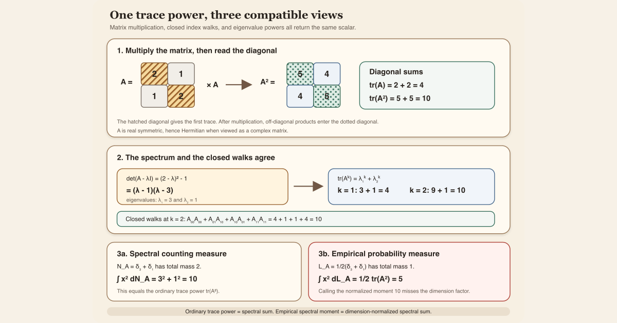
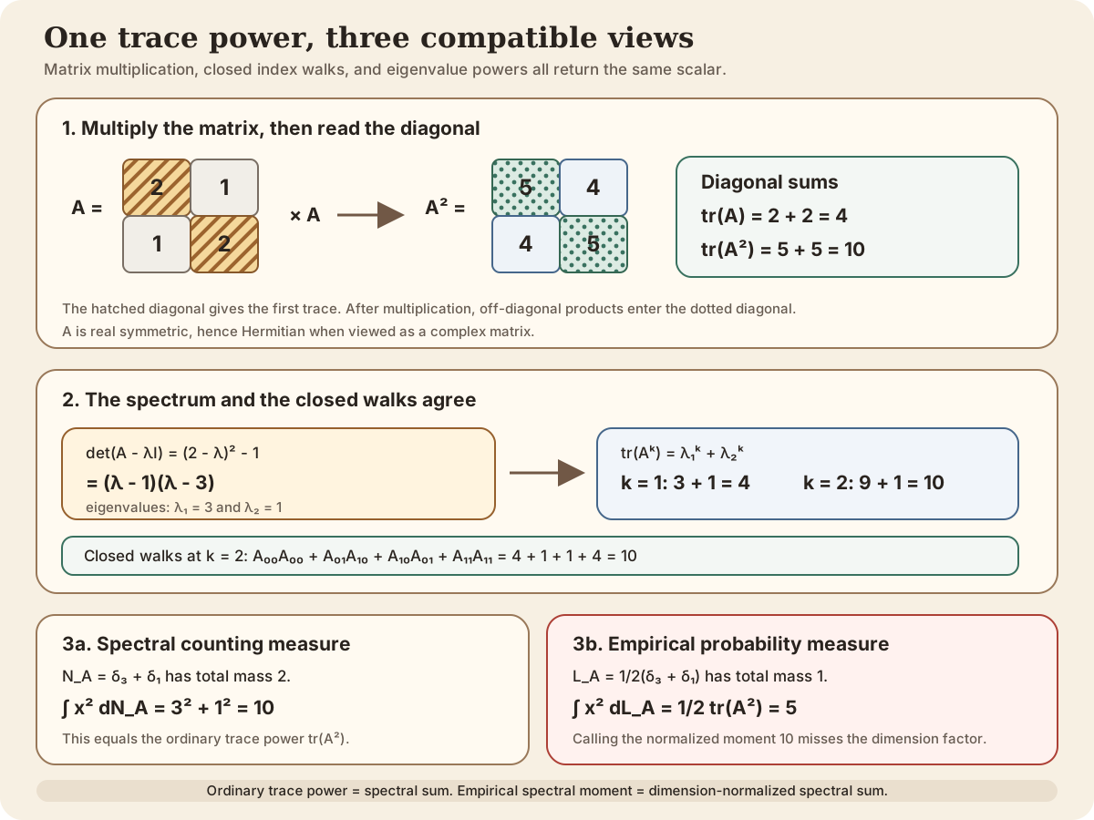
\[ A= \begin{bmatrix} 2&1\\ 1&2 \end{bmatrix}. \]

This matrix is real symmetric, so as a complex matrix it is Hermitian . Its first power is \(A\), and its ordinary matrix trace is

\[ \operatorname{tr}(A)=2+2=4. \]

Now multiply it by itself:

\[ \begin{aligned} A^2 &= \begin{bmatrix} 2&1\\ 1&2 \end{bmatrix} \begin{bmatrix} 2&1\\ 1&2 \end{bmatrix}\\ &= \begin{bmatrix} 2\cdot2+1\cdot1 & 2\cdot1+1\cdot2\\ 1\cdot2+2\cdot1 & 1\cdot1+2\cdot2 \end{bmatrix}\\ &= \begin{bmatrix} 5&4\\ 4&5 \end{bmatrix}. \end{aligned} \]

Therefore

\[ \operatorname{tr}(A^2)=5+5=10. \]

The off-diagonal entries did not enter \(\operatorname{tr}(A)\) directly, but they did enter the diagonal of \(A^2\). Trace powers therefore retain interactions absent from the first trace.

Compute the eigenvalues

The characteristic polynomial is

\[ \begin{aligned} \det(A-\lambda I) &= \det \begin{bmatrix} 2-\lambda&1\\ 1&2-\lambda \end{bmatrix}\\ &=(2-\lambda)^2-1\\ &=\lambda^2-4\lambda+3\\ &=(\lambda-1)(\lambda-3). \end{aligned} \]

Thus the eigenvalues are

\[ \lambda_1=3, \qquad \lambda_2=1. \]

The vector \((1,1)\) is an eigenvector for \(3\), and \((1,-1)\) is an eigenvector for \(1\). After normalizing those vectors, the spectral decomposition is

\[ A= \frac1{\sqrt2} \begin{bmatrix} 1&1\\ 1&-1 \end{bmatrix} \begin{bmatrix} 3&0\\ 0&1 \end{bmatrix} \frac1{\sqrt2} \begin{bmatrix} 1&1\\ 1&-1 \end{bmatrix}^{*}. \]

Here \(^{*}\) denotes conjugate transpose. Raising the decomposition to the \(k\)-th power raises only the eigenvalues:

\[ A^k =Q \begin{bmatrix} 3^k&0\\ 0&1^k \end{bmatrix} Q^*. \]

Trace is unchanged by this unitary change of basis, so

\[ \operatorname{tr}(A^k)=3^k+1^k. \]

The first two cases reproduce the entry calculations:

\[ \operatorname{tr}(A)=3+1=4, \qquad \operatorname{tr}(A^2)=3^2+1^2=10. \]

At \(k=0\), \(A^0=I_2\), so \(\operatorname{tr}(A^0)=2=3^0+1^0\). The exponent-zero case counts the dimension.

The two by two Hermitian matrix with rows two one and one two is squared to obtain rows five four and four five. Its traces are four and ten. A characteristic-polynomial calculation gives eigenvalues three and one, whose first and second powers sum to the same traces. A closed-walk expansion gives four plus one plus one plus four. The bottom compares unnormalized spectral counting moment ten with normalized empirical spectral moment five. — FigureFinding: for \(A=\left[\begin{smallmatrix}2&1\\1&2\end{smallmatrix}\right]\), direct multiplication gives \(A^2=\left[\begin{smallmatrix}5&4\\4&5\end{smallmatrix}\right]\), so \(\operatorname{tr}(A)=4\) and \(\operatorname{tr}(A^2)=10\). The characteristic polynomial factors as \((\lambda-1)(\lambda-3)\), and the spectral sums give \(3+1=4\) and \(3^2+1^2=10\). The closed two-step index walks give the same \(4+1+1+4=10\). The spectral counting measure has second moment \(10\); the empirical spectral probability measure divides by dimension \(2\) and has second moment \(5\). Patterns mark the relevant diagonal entries without relying on color.

Why the identity holds

For a finite Hermitian matrix, the spectral theorem gives

\[ A=QDQ^*, \]

where \(Q\) is unitary and \(D=\operatorname{diag}(\lambda_1,\ldots,\lambda_n)\). Hence

\[ A^k=QD^kQ^*. \]

Cyclicity of trace removes the change of basis:

\[ \begin{aligned} \operatorname{tr}(A^k) &=\operatorname{tr}(QD^kQ^*)\\ &=\operatorname{tr}(D^kQ^*Q)\\ &=\operatorname{tr}(D^k)\\ &=\sum_{i=1}^n\lambda_i^k. \end{aligned} \]

Hermiticity makes all eigenvalues real, so every trace power is real. For a general finite complex matrix the same eigenvalue-sum identity remains true when eigenvalues are counted with algebraic multiplicity, even if the matrix is not diagonalizable. The Hermitian case is especially transparent because it has an orthonormal eigenbasis.

The closed-walk view

Matrix multiplication gives a second interpretation. For \(k\ge1\),

\[ \operatorname{tr}(A^k) {} = \sum_{i_0,\ldots,i_{k-1}} A_{i_0i_1}A_{i_1i_2}\cdots A_{i_{k-1}i_0}. \]

Each term follows an index path and returns to its starting index. For the two-by-two example at \(k=2\), the four closed walks contribute

\[ \begin{aligned} \operatorname{tr}(A^2) &=A_{00}A_{00}+A_{01}A_{10} +A_{10}A_{01}+A_{11}A_{11}\\ &=2\cdot2+1\cdot1+1\cdot1+2\cdot2\\ &=10. \end{aligned} \]

This coordinate formula drives the random-matrix moment method. When entries are random, centering, independence, and covariance decide which closed-index patterns survive after taking an expectation. The trace packages a large entrywise expansion into one basis-independent spectral statistic.

Exactly which spectral moment?

Let the eigenvalues of an \(n\times n\) Hermitian matrix be \(\lambda_1,\ldots,\lambda_n\). The spectral counting measure

\[ N_A=\sum_{i=1}^n\delta_{\lambda_i} \]

has total mass \(n\). Its \(k\)-th raw moment is exactly the ordinary trace power:

\[ \int_{\mathbb R}x^k\,dN_A(x) =\sum_{i=1}^n\lambda_i^k =\operatorname{tr}(A^k). \]

The empirical spectral measure

\[ L_A=\frac1n\sum_{i=1}^n\delta_{\lambda_i} \]

is instead a probability measure. Its \(k\)-th moment is

\[ \int_{\mathbb R}x^k\,dL_A(x) =\frac1n\operatorname{tr}(A^k). \]

For the example, \(N_A=\delta_3+\delta_1\), while \(L_A=\tfrac12(\delta_3+\delta_1)\). Therefore

\[ \int x^2\,dN_A=10, \qquad \int x^2\,dL_A=5. \]

Calling \(10\) the second moment of the empirical probability measure misses the factor \(1/2\). The number \(10\) is the second moment of the spectral counting measure and the ordinary trace power.

Random matrices add an outcome variable

For a finite random matrix

\[ X:\Omega\longrightarrow\mathbb C^{n\times n}, \]

the project defines the trace-power observable

\[ \omega\longmapsto\operatorname{tr}\bigl(X(\omega)^k\bigr). \]

One outcome \(\omega\) selects one realized matrix and one trace-power value. The observable itself is the entire scalar-valued function on outcomes. Its expectation , when licensed by a probability measure and an integrability proof, is

\[ \mathbb E\!\left[\operatorname{tr}(X^k)\right]. \]

Measurability and integrability are separate. The project’s elementary observables module proves that a measurable finite matrix-valued map has a measurable trace-power observable. It does not claim that every such observable is integrable. The ensemble-specific GUE moment module later proves integrability and computes the first two expected trace powers.

The finite matrix trace moment entry develops that probability layer. The empirical-spectrum module then relates normalized trace powers to spectral probability moments.

In Lean: from a realized matrix to a scalar

One idea, three languages Read across, then read the syntax map

A human says

At outcome omega, raise the realized matrix X(omega) to the natural-number power k and add the diagonal entries.

On paper

\(\omega\longmapsto\operatorname{tr}\!\left(X(\omega)^k\right).\)

In Lean

RandomMatrix.tracePower X k

Syntax map

RandomMatrix is the project namespace containing the observable, not an extra proof that X is random in a probabilistic sense.
X : RandomMatrix Ω ι ι ℂ is a function from outcomes to square complex matrices. Repeating ι makes the row and column index types agree.
k : ℕ is a natural-number exponent, including zero.
RandomMatrix.tracePower X k is a function Ω → ℂ. A human applies it to one outcome by typing RandomMatrix.tracePower X k ω.
After unfolding the definition, the exact Lean expression is Matrix.trace ((X ω) ^ k).
X ω is function application, corresponding to \(X(\omega)\).
^ k is matrix exponentiation. Parentheses around X ω make the object being powered explicit.
Matrix.trace adds the finite diagonal and returns one complex scalar.

The next theorem moves from algebra to the measurable-observable layer:

One idea, three languages Read across, then read the syntax map

A human says

If X is a measurable finite square complex matrix-valued function, then every trace-power observable of X is measurable.

On paper

\(X\text{ measurable}\Longrightarrow[\omega\mapsto\operatorname{tr}(X(\omega)^k)]\text{ measurable}.\)

In Lean

RandomMatrix.measurable_tracePower hX k

Syntax map

hX : Measurable X names the hypothesis that the matrix-valued function is measurable.
measurable_tracePower first proves matrix powers measurable by induction on k, then applies measurability of finite trace.
The theorem establishes no expectation or integrability claim.
For an everywhere-Hermitian realization, the separate theorem hX.tracePower_im_eq_zero k ω proves that the complex result has imaginary part zero.

The exact checked project definition and measurability theorem are:

def tracePower [Fintype ι] [DecidableEq ι]
    (X : RandomMatrix Ω ι ι ℂ) (k : ℕ) : Ω → ℂ :=
  fun ω ↦ Matrix.trace ((X ω) ^ k)

theorem measurable_tracePower [Fintype ι] [DecidableEq ι]
    {X : RandomMatrix Ω ι ι ℂ} (hX : Measurable X) (k : ℕ) :
    Measurable (tracePower X k) := by
  change Measurable fun ω ↦ Matrix.trace ((X ω) ^ k)
  exact measurable_trace (measurable_matrixPow hX k)

The typeclass [Fintype ι] supplies the finite diagonal over which trace sums. [DecidableEq ι] supports the finite square matrix identity used at exponent zero and the matrix-power API.

Standalone tutorial

Standalone tutorial. This worksheet imports only Lean’s Std library. It does not import Mathlib or this project. It verifies the concrete integer arithmetic, not the general spectral theorem.

Save the following as TracePowerScratch.lean:

import Std

structure Matrix2 where
  a00 : Int
  a01 : Int
  a10 : Int
  a11 : Int
deriving Repr

namespace Matrix2

def mul (A B : Matrix2) : Matrix2 :=
  { a00 := A.a00 * B.a00 + A.a01 * B.a10
    a01 := A.a00 * B.a01 + A.a01 * B.a11
    a10 := A.a10 * B.a00 + A.a11 * B.a10
    a11 := A.a10 * B.a01 + A.a11 * B.a11 }

def trace (A : Matrix2) : Int :=
  A.a00 + A.a11

end Matrix2

def A : Matrix2 :=
  { a00 := 2, a01 := 1, a10 := 1, a11 := 2 }

def A2 : Matrix2 :=
  Matrix2.mul A A

#eval A2
#eval Matrix2.trace A
#eval Matrix2.trace A2
#eval (3 : Int) ^ 2 + (1 : Int) ^ 2

Run it with:

elan run leanprover/lean4:v4.32.0 lean TracePowerScratch.lean

The four evaluations should display the squared matrix with entries \(5,4,4,5\), then \(4\), \(10\), and \(10\). This scratch model deliberately uses a concrete four-field structure. It teaches multiplication and trace without serving as a replacement for Mathlib’s generic Matrix API.

Project declaration workflow

Try it in the repository NonlinearDynamics/Random/RandomMatrices/Observables.lean

Full project check. This uses the repository’s pinned Lean and Mathlib dependencies and may require substantial disk space and memory. The authoritative source is formalization/NonlinearDynamics/Random/RandomMatrices/Observables.lean. A human can type this worksheet in a temporary Lean file:

import NonlinearDynamics.Random.RandomMatrices.Observables

#check NonlinearDynamics.Random.RandomMatrix.tracePower
#check NonlinearDynamics.Random.RandomMatrix.measurable_matrixPow
#check NonlinearDynamics.Random.RandomMatrix.measurable_tracePower
#check NonlinearDynamics.Random.RandomMatrix.IsHermitianEverywhere.tracePower_im_eq_zero
#check NonlinearDynamics.Random.HermitianRandomMatrix.measurable_tracePower
#check NonlinearDynamics.Random.HermitianRandomMatrix.tracePower_im_eq_zero

Each #check asks the pinned Lean elaborator to display the exact type of a project declaration. It does not rerun the hand calculation and does not prove a new theorem. The full-project command below checks the authoritative module.

Full project check, from the repository root

cd formalization
lake env lean -DwarningAsError=true NonlinearDynamics/Random/RandomMatrices/Observables.lean

Resource note: this exact file uses the repository's pinned Lean and Mathlib dependencies. Initial project setup can require substantial disk space and build time. For a lightweight first step on macOS or Linux, use the page's standalone Lean-core or Std tutorial.

Normalization and other boundaries

Tempting shortcut	What is wrong	Correct repair
“Trace power means entrywise powers”	Matrix multiplication mixes rows and columns	Form the matrix power \(A^k\), then take trace
“Off-diagonal entries never matter”	They contribute to diagonal entries after multiplication	Expand at least one matrix product
“Trace power is one eigenvalue power”	Trace sums all eigenvalues with multiplicity	Use \(\sum_i\lambda_i^k\)
“The empirical spectral moment equals the ordinary trace”	The empirical measure has mass one rather than \(n\)	Divide by dimension
“Scaling the trace is the same as scaling the matrix”	Matrix scaling is raised to the \(k\)-th power	Track both the \(n^{-1}\) and \(n^{-k/2}\) factors
“Measurable implies integrable”	A measurable observable can have divergent tails	Prove integrability before taking a finite expectation
“A real trace power proves the matrix is Hermitian”	Non-Hermitian matrices can have real trace powers	Use Hermiticity as a separate structural hypothesis
“All trace powers reconstruct every matrix”	Trace powers determine spectral information, not eigenvectors or a basis	Separate spectrum from full matrix data

Where to continue

Read matrix trace for the diagonal sum and its similarity invariance. Read empirical spectral measure for the dimension-normalized spectral probability measure. Read finite matrix trace moment for the integrability and expectation layer, and random matrix for the outcome-dependent matrix itself.

The chapter First Exact Finite Gaussian Unitary Ensemble Trace Moments computes the first two expected trace powers in the project’s finite Wigner-scaled GUE. The chapter Finite GUE Empirical Spectral Laws and Normalized Moments then identifies their normalized spectral-measure counterparts.

References

Mathlib contributors. Matrix trace, Mathlib 4 documentation. This official implementation reference documents the finite trace operation used by RandomMatrix.tracePower.

Terence Tao. Topics in Random Matrix Theory, Graduate Studies in Mathematics 132, American Mathematical Society, 2012. This reference develops trace moments, closed-walk expansions, and the random-matrix moment method.

Roger A. Horn and Charles R. Johnson. Matrix Analysis, second edition, Cambridge University Press, 2012. This is a standard source for Hermitian spectral decomposition, trace, eigenvalue multiplicity, and matrix powers.

Nonlinear Dynamics in Lean contributors. Observables.lean, the checked project source for trace-power definition, measurability, and Hermitian reality.