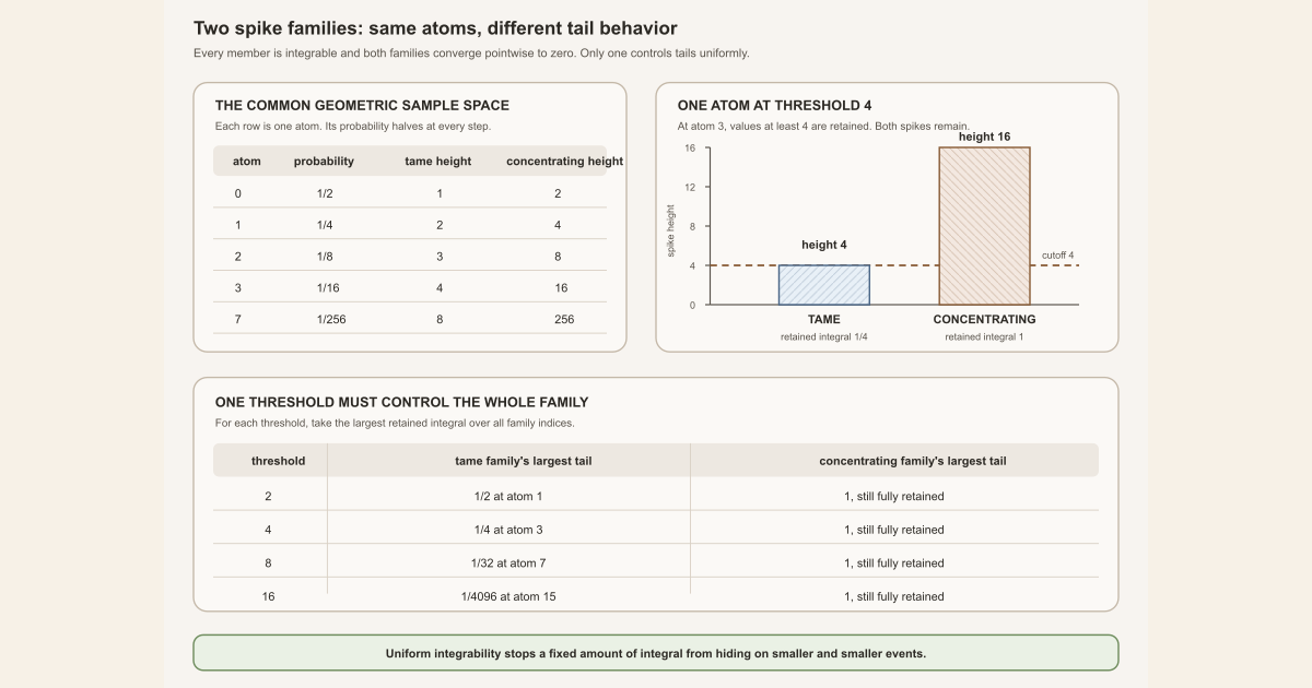
Start with two spike families
Take the sample space
\[ \Omega=\{0,1,2,\ldots\} \]and declare every subset of \(\Omega\) measurable. On this discrete measurable space, assign the point \(k\) probability
\[ \mu(\{k\})=2^{-(k+1)}. \]The geometric series sums to one, so \(\mu\) is a probability measure . The singleton \(A_n=\{n\}\) is an event , and its probability \(2^{-(n+1)}\) becomes very small as \(n\) grows.
Define two real-valued function families on this same space:
\[ F_n(k)=(n+1)\mathbf 1_{A_n}(k), \qquad G_n(k)=2^{n+1}\mathbf 1_{A_n}(k). \]Here \(\mathbf 1_{A_n}\) is one on \(A_n\) and zero elsewhere. Thus each function has exactly one nonzero value. Its integral is
\[ \text{height of the spike}\times\text{probability of its supporting atom}. \]The first values are completely explicit:
| index \(n\) | atom probability \(\mu(A_n)\) | height of \(F_n\) | \(\int |F_n|\,d\mu\) | height of \(G_n\) | \(\int |G_n|\,d\mu\) | |—:|—:|—:|—:|—:|—:| | \(0\) | \(1/2\) | \(1\) | \(1/2\) | \(2\) | \(1\) | | \(1\) | \(1/4\) | \(2\) | \(1/2\) | \(4\) | \(1\) | | \(2\) | \(1/8\) | \(3\) | \(3/8\) | \(8\) | \(1\) | | \(3\) | \(1/16\) | \(4\) | \(1/4\) | \(16\) | \(1\) | | \(7\) | \(1/256\) | \(8\) | \(1/32\) | \(256\) | \(1\) |
Every \(F_n\) and every \(G_n\) is integrable because it has a finite integral. For a real function \(H\), its \(L^1\) norm is \(\lVert H\rVert_1=\int |H|\,d\mu\). Both families even have a common \(L^1\)-norm bound: the norms of the \(F_n\) are at most \(1/2\), while every \(G_n\) has norm exactly \(1\). Nevertheless, only the \(F_n\) family is uniformly integrable.
There is also pointwise convergence in both cases. Fix \(k\in\Omega\). The value \(F_n(k)\), or \(G_n(k)\), is nonzero only once, when \(n=k\). It is zero for every later index, so
\[ F_n(k)\longrightarrow 0, \qquad G_n(k)\longrightarrow 0. \]The \(G_n\) family is the warning: pointwise convergence and bounded \(L^1\) norms still do not force \(L^1\) convergence. Indeed,
\[ \lVert F_n\rVert_1=\frac{n+1}{2^{n+1}}\longrightarrow0, \qquad \lVert G_n\rVert_1=1. \]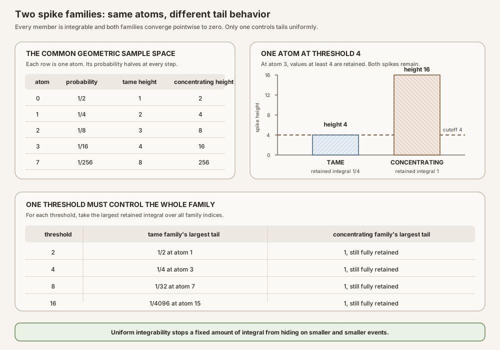
Compute what the common threshold measures
For a family \(H_n\), define its worst large-value tail at threshold \(C\) by
\[ \tau_H(C) {}=\sup_n\int_{\{|H_n|\ge C\}}|H_n|\,d\mu. \]The inequality is inclusive: a value exactly equal to \(C\) remains in the tail. Uniform integrability at exponent one asks for one threshold \(C\) that works for every family index after a tolerance has been requested:
\[ \forall\varepsilon\gt0\;\exists C\ge0\;\forall n, \qquad \int_{\{|H_n|\ge C\}}|H_n|\,d\mu\le\varepsilon. \]The decisive order is
\[ \boxed{\forall\varepsilon\;\exists C\;\forall n.} \]A separate threshold \(C_n\) for each function would merely recover individual integrability. The threshold must be shared by the whole family.
For \(F_n\), let \(m=n+1\). Its only possible nonzero tail contribution is
\[ \int_{\{|F_n|\ge C\}}|F_n|\,d\mu {}= \begin{cases} m/2^m,&m\ge C,\\ 0,&m\lt C. \end{cases} \]The sequence \(m/2^m\) is nonincreasing for positive integers \(m\) and is strictly decreasing after \(m=1\). At an integer threshold \(M\ge2\), the largest surviving contribution therefore occurs at \(m=M\):
| common threshold \(C\) | largest \(F_n\) tail | index attaining it | largest \(G_n\) tail |
|---|---|---|---|
| \(2\) | \(2/4=1/2\) | \(n=1\) | \(1\) |
| \(4\) | \(4/16=1/4\) | \(n=3\) | \(1\) |
| \(8\) | \(8/256=1/32\) | \(n=7\) | \(1\) |
| \(16\) | \(16/65536=1/4096\) | \(n=15\) | \(1\) |
Because \(M/2^M\to0\), given any \(\varepsilon\gt0\) we can choose \(M\) with \(M/2^M\lt\varepsilon\). The threshold \(C=M\) then makes every \(F_n\) tail smaller than \(\varepsilon\). Thus the \(F_n\) are uniformly integrable even though their spike heights \(n+1\) are unbounded. Uniform integrability does not mean a common pointwise height bound.
For \(G_n\), the spike height is \(2^{n+1}\) and its supporting atom has probability \(2^{-(n+1)}\). Their product is always one. Given any finite threshold \(C\), choose \(n\) with \(2^{n+1}\ge C\). The whole spike remains, so
\[ \int_{\{|G_n|\ge C\}}|G_n|\,d\mu=1. \]Consequently \(\tau_G(C)=1\) for every finite \(C\). No threshold can meet, for example, the tolerance \(\varepsilon=1/2\).
The same failure appears in small-set language. The events \(A_n\) satisfy \(\mu(A_n)\to0\), but
\[ \int_{A_n}|G_n|\,d\mu=1 \qquad\text{for every }n. \]Mass is concentrating on smaller and smaller events without becoming smaller in the integral. This is exactly what uniform integrability forbids.
Random Matrix Theory milestone 27 (RMT-27) needs that uniform control to upgrade almost-everywhere convergence of Birkhoff averages to convergence in \(L^1\). The complete checked narrative is Identifying the Finite-Measure Birkhoff Limit in Lean. The textbook chapter is Birkhoff Limits, Invariant Sigma Algebras, and Conditional Expectation.
The two Mathlib predicates
Mathlib deliberately distinguishes two related notions. Let \(\Omega\) be a
measurable space, let \(\mu\) be a measure on it, let \(I\) be an index type,
and let \(F_i:\Omega\to E\) be a family of functions into a normed additive
space \(E\). For an extended nonnegative exponent \(p\), the predicate
UnifIntegrable F p μ is the small-set condition:
The exact pinned source declaration, with Mathlib’s local type-variable names, is:
def UnifIntegrable {_ : MeasurableSpace α} (f : ι → α → β)
    (p : ℝ≥0∞) (μ : Measure α) : Prop :=
  ∀ ⦃ε : ℝ⦄ (_ : 0 < ε), ∃ (δ : ℝ) (_ : 0 < δ), ∀ i s,
    MeasurableSet s → μ s ≤ ENNReal.ofReal δ →
      eLpNorm (s.indicator (f i)) p μ ≤ ENNReal.ofReal ε
In words: for every positive tolerance \(\varepsilon\), there is one positive
measure scale \(\delta\) such that every family member has \(L^p\) norm at
most \(\varepsilon\) when restricted to every measurable set of measure at
most \(\delta\). The function
S.indicator (F i) agrees with \(F_i\) on \(S\) and is zero
outside \(S\). The extended value eLpNorm is Mathlib’s
extended-nonnegative \(L^p\) norm.
The capitalized predicate used directly by RMT-27 is stronger:
def UniformIntegrable {_ : MeasurableSpace α} (f : ι → α → β)
    (p : ℝ≥0∞) (μ : Measure α) : Prop :=
  (∀ i, AEStronglyMeasurable (f i) μ) ∧
  UnifIntegrable f p μ ∧
  ∃ C : ℝ≥0, ∀ i, eLpNorm (f i) p μ ≤ C
It bundles three facts:
- every member is strongly measurable almost everywhere;
- the small-set control is uniform across the family; and
- all full \(L^p\) norms share one finite bound.
Mathlib’s source calls the first predicate the measure-theory sense and the
capitalized predicate the probability-theory sense. The names do not impose
probability normalization. RMT-27 uses UniformIntegrable on an
arbitrary finite measure, whose total mass may differ from one.
The theorem that upgrades convergence uses the small-set component. A proof
h : UniformIntegrable F 1 μ provides it through
h.unifIntegrable, while also making each family member an
\(L^1\) function through h.memLp.
Equivalent tail control on a finite measure space
For finite \(\mu\) and \(1\le p\lt\infty\), Mathlib proves an equivalent
large-value-tail formulation. Up to the almost-everywhere measurability
clause, UniformIntegrable F p μ says that for every
\(\varepsilon\gt0\), there is one nonnegative threshold \(C\) such that
The indicator \(\mathbf 1_A\) keeps a function on the set \(A\) and replaces it by zero elsewhere. At \(p=1\) for real functions, the displayed norm is the integral of \(|F_i|\) over the part where \(|F_i|\) is at least \(C\). The important order is
\[ \forall\varepsilon\gt0\ \exists C\ge0\ \forall i. \]Allowing a separate threshold \(C_i\) for each member would say only that each function is integrable. Uniform integrability requires a single threshold after the tolerance is fixed.
The small-set and tail forms express the same obstruction from opposite directions. One prevents mass from hiding on sets of vanishing measure. The other prevents mass from escaping to values of growing magnitude. Finite total measure is part of Mathlib’s equivalence theorem and should not be erased when using that API.
Why measure-preserving orbit translates are uniform
Let \(T:\Omega\to\Omega\) preserve a finite measure \(\mu\), and let \(f:\Omega\to\mathbb R\) be integrable. The orbit-translate family is
\[ F_i(\omega)=f(T^i\omega), \qquad i\in\mathbb N. \]Measure preservation says that the pushforward of \(\mu\) through every iterate \(T^i\) is again \(\mu\). Therefore every \(F_i\) has the same pushforward distribution as \(f\). When \(\mu\) is probability normalized, that pushforward is a probability law ; on the module’s general finite measure it is a finite measure with the same total mass as \(\mu\). In Lean, RMT-27 first proves
theorem identDistrib_orbit_iterate
    (hT : MeasurePreserving T μ μ) (hf : AEMeasurable f μ) (i : ℕ) :
    IdentDistrib (fun ω ↦ f ((T^[i]) ω)) f μ μ
Identical distribution means that every measurable test event in the target has the same measure under both functions. It transfers \(L^1\) norms and all large-value-tail norms. Mathlib packages the family-wide consequence:
MemLp.uniformIntegrable_of_identDistrib
RMT-27 specializes it at \(p=1\) to obtain
theorem uniformIntegrable_orbit_iterate
    [IsFiniteMeasure μ]
    (hT : MeasurePreserving T μ μ) (hf : Integrable f μ) :
    UniformIntegrable (fun i ω ↦ f ((T^[i]) ω)) 1 μ
No independence assumption appears. Orbit translates are usually highly dependent because they are values along the same trajectory. Identical distribution is sufficient for this uniform-integrability step.
The finite-measure premise belongs to the pinned Mathlib theorem used here. It does not say that identical distribution is conceptually meaningless on every infinite-measure space; it records the checked route of this module.
Cesaro averaging preserves the control
The positive-time Birkhoff averages are Cesaro means of the translates:
\[ A_nf {} = \frac1n\sum_{i=0}^{n-1}F_i. \]Uniform integrability must survive this averaging operation before it can be combined with RMT-26’s pointwise convergence theorem. Mathlib provides exactly that closure:
theorem uniformIntegrable_average
    (hp : 1 ≤ p) (hF : UniformIntegrable F p μ) :
    UniformIntegrable
      (fun n ↦ (n : ℝ)⁻¹ • ∑ i ∈ Finset.range n, F i) p μ
The proof uses the triangle inequality for restricted \(L^p\) norms and the shared full-norm bound. At horizon zero, Lean’s inverse convention gives the zero average. Adding this one zero function causes no problem and lets the result cover the complete natural-number sequence without a special index type.
RMT-27 aligns Mathlib’s generic average with the project’s
birkhoffAverage definition and exposes
theorem uniformIntegrable_birkhoffAverage
    [IsFiniteMeasure μ]
    (hT : MeasurePreserving T μ μ) (hf : Integrable f μ) :
    UniformIntegrable (fun n ↦ birkhoffAverage ℝ T f n) 1 μ
Uniform integrability of the averages does not yet prove that they converge. It provides stability once a convergence mode such as almost-everywhere convergence is supplied.
The Vitali bridge in RMT-27
RMT-26 proves that for almost every \(\omega\), the sequence
\(A_nf(\omega)\) converges to the selected total representative
\(L(\omega)=\operatorname{birkhoffLimit}(T,f,\omega)\). Mathlib’s
UniformIntegrable.integrable_of_ae_tendsto first shows that
\(L\) is integrable.
Then the finite-measure Vitali theorem
tendsto_Lp_finite_of_tendsto_ae
combines:
- almost-everywhere strong measurability of every average;
- membership of the limit in \(L^1\);
UnifIntegrablecontrol inherited from the strongerUniformIntegrableresult; and- almost-everywhere pointwise convergence.
Its conclusion at \(p=1\) is
\[ \left\lVert A_nf-L\right\rVert_{L^1(\mu)}\longrightarrow0. \]That is a stronger conclusion than RMT-26’s pointwise convergence, but it is proved rather than assumed. It allows the integral over every measurable set to pass to the limit. RMT-27 applies this continuity on exactly invariant sets and then invokes conditional expectation uniqueness.
The logical chain is therefore
\[ \begin{aligned} \text{measure-preserving translates} &\Longrightarrow \text{identical distribution} \\ &\Longrightarrow \text{uniform integrability of translates} \\ &\Longrightarrow \text{uniform integrability of averages} \\ &\mathrel{+} \text{almost-everywhere convergence} \\ &\Longrightarrow L^1\text{ convergence} \\ &\Longrightarrow \text{passage of invariant-set integrals}. \end{aligned} \]Every arrow is represented by a checked theorem. Pointwise convergence alone would skip the indispensable middle of the argument.
In Lean: read the small-set definition
UnifIntegrable F p μ∀ ⦃ε : ℝ⦄introduces every real tolerance. The braces make this argument implicit when the predicate is applied.0 < εand0 < δrecord positivity.∀ i Splaces the family index and set after the same cutoff. That position is the family-wide quantifier.MeasurableSet Sis the regularity needed for restriction.μ S ≤ ENNReal.ofReal δcompares the extended-nonnegative measure with a real cutoff converted byENNReal.ofReal.S.indicator (F i)is the member restricted to \(S\).
The predicate controls where \(L^p\) mass may hide. It does not mention pointwise convergence or choose a candidate limit.
In Lean: use the finite-measure tail criterion
uniformIntegrable_iff hp hp'[IsFiniteMeasure μ]is an instance required by this theorem.hp : 1 ≤ prules out exponents below one.hp’ : p ≠ ∞rules out the top exponent.C : ℝ≥0makes the threshold nonnegative by type.{ x | C ≤ ‖F i x‖₊ }is the inclusive large-value event.‖F i x‖₊is the nonnegative-real norm of the value.
This bridge is the exact Mathlib result behind the spike calculation. The mathematics on this page used \(p=1\), but the theorem is parameterized by every finite extended-nonnegative exponent \(p\) with \(1\le p\).
In Lean: orbit translates share one control
uniformIntegrable_orbit_iterate hT hfhT : MeasurePreserving T μ μcertifies measurability of \(T\) and preservation of the same measure \(\mu\).hf : Integrable f μis the \(L^1\) premise.T^[i]is Lean notation for the \(i\)-fold iterate of \(T\).- The result is
UniformIntegrable (fun i ω ↦ f ((T^[i]) ω)) 1 μ. - No ergodicity, mixing, or independence premise occurs.
The complete project proof is short because the pinned identical-distribution theorem performs the family-wide analytic step:
theorem uniformIntegrable_orbit_iterate
    [IsFiniteMeasure μ]
    (hT : MeasurePreserving T μ μ) (hf : Integrable f μ) :
    UniformIntegrable (fun i ω ↦ f ((T^[i]) ω)) 1 μ := by
  apply ProbabilityTheory.MemLp.uniformIntegrable_of_identDistrib
    (f := fun i ω ↦ f ((T^[i]) ω)) (j := 0) (p := 1)
    le_rfl ENNReal.one_ne_top
    (by simpa only [Function.iterate_zero, id_eq] using
      (memLp_one_iff_integrable.mpr hf))
  intro i
  simpa only [Function.iterate_zero, id_eq] using
    (identDistrib_orbit_iterate hT hf.aemeasurable i)
Index zero is the reference member because \(T^0\) is the identity. The last line proves that every other member has the same distribution as that reference.
A tiny standalone Lean worksheet a human can type
Standalone tutorial. The following file records a retained integral as a pair
(numerator, denominator). For example, (4, 16)
means the exact value \(4/16\). It checks the spike arithmetic and the
inclusive threshold rule without importing Mathlib, defining a measure, or
proving the infinite-family supremum.
Save this as UniformIntegrabilityTutorial.lean:
import Std

namespace UniformIntegrabilityTutorial

def atomDenominator (n : Nat) : Nat :=
  2 ^ (n + 1)

def tameHeight (n : Nat) : Nat :=
  n + 1

def concentratingHeight (n : Nat) : Nat :=
  atomDenominator n

def tailNumerator (height : Nat → Nat) (threshold n : Nat) : Nat :=
  if threshold ≤ height n then height n else 0

def tailFraction (height : Nat → Nat) (threshold n : Nat) : Nat × Nat :=
  (tailNumerator height threshold n, atomDenominator n)

#eval (List.range 5).map (tailFraction tameHeight 4)
#eval (List.range 5).map (tailFraction concentratingHeight 4)
#eval [tailFraction tameHeight 2 1, tailFraction tameHeight 4 3,
  tailFraction tameHeight 8 7, tailFraction tameHeight 16 15]
#eval [tailFraction concentratingHeight 2 0,
  tailFraction concentratingHeight 4 1,
  tailFraction concentratingHeight 8 2,
  tailFraction concentratingHeight 16 3]

example : tailFraction tameHeight 4 2 = (0, 8) := by decide
example : tailFraction tameHeight 4 3 = (4, 16) := by decide
example : tailFraction tameHeight 8 7 = (8, 256) := by decide
example : tailFraction concentratingHeight 4 1 = (4, 4) := by decide
example : tailFraction concentratingHeight 16 3 = (16, 16) := by decide

end UniformIntegrabilityTutorial
From the directory containing the file, type:
source "$HOME/.elan/env"
elan run leanprover/lean4:v4.32.0 lean UniformIntegrabilityTutorial.lean
This exact worksheet was executed successfully with Lean 4.32.0 while editing
this page. Its first output was
[(0, 2), (0, 4), (0, 8), (4, 16), (5, 32)]. The second was
[(0, 2), (4, 4), (8, 8), (16, 16), (32, 32)]. The third was
[(2, 4), (4, 16), (8, 256), (16, 65536)], and the fourth was
[(2, 2), (4, 4), (8, 8), (16, 16)]. These are the
decisive table entries. The tame numerators have rapidly growing denominators,
while every concentrating fraction has equal numerator and denominator. This
bounded worksheet does not download or build the project or Mathlib.
Try the exact declarations in the repository
Full project check. This uses the repository’s pinned Lean and Mathlib dependencies and may require substantial disk space and memory. Create a project scratch file containing the following commands, or compare them with the named module:
import NonlinearDynamics.Random.RandomCocycles.PointwiseBirkhoffLimit

#check MeasureTheory.UnifIntegrable
#check MeasureTheory.UniformIntegrable
#check MeasureTheory.uniformIntegrable_iff
#check MeasureTheory.uniformIntegrable_average
#check ProbabilityTheory.MemLp.uniformIntegrable_of_identDistrib
#check MeasureTheory.UniformIntegrable.integrable_of_ae_tendsto
#check MeasureTheory.tendsto_Lp_finite_of_tendsto_ae
#check NonlinearDynamics.Random.RandomCocycles.identDistrib_orbit_iterate
#check NonlinearDynamics.Random.RandomCocycles.uniformIntegrable_orbit_iterate
#check NonlinearDynamics.Random.RandomCocycles.uniformIntegrable_birkhoffAverage
#check NonlinearDynamics.Random.RandomCocycles.integrable_birkhoffLimit
#check NonlinearDynamics.Random.RandomCocycles.tendsto_L1_birkhoffAverage_birkhoffLimit
Each #check asks the pinned elaborator for an existing declaration
and its exact type. The full-project command below checks the complete
PointwiseBirkhoffLimit.lean module. It uses the repository’s
pinned Lean and Mathlib dependencies.
cd formalization
lake env lean -DwarningAsError=true NonlinearDynamics/Random/RandomCocycles/PointwiseBirkhoffLimit.lean
Resource note: this exact file uses the repository's
pinned Lean and Mathlib dependencies. Initial project setup can require
substantial disk space and build time. For a lightweight first step on
macOS or Linux, use the page's standalone Lean-core or Std
tutorial.
Boundaries and nonclaims
- A finite family is different. A genuinely finite collection of \(L^p\) functions is uniformly integrable under Mathlib’s usual \(1\le p\lt\infty\) assumptions. The escaping-spike obstruction needs new behavior to keep appearing along an infinite family.
- A common pointwise bound is sufficient, not necessary. On a finite measure space, a common height bound eventually makes every large-value tail empty. The tame \(F_n\) family is uniformly integrable even though its heights \(n+1\) are unbounded.
- Uniform \(L^1\)-norm boundedness is not enough. The family \(G_n\) above has norm exactly one and still fails uniform integrability.
- Individual integrability is not uniform integrability. Letting the threshold depend on the family index removes the required single threshold that must work uniformly over the family.
- Uniform integrability does not imply pointwise convergence. It controls mass escape. A separate convergence hypothesis is still required by the Vitali step.
- Pointwise convergence does not imply norm convergence. The same \(G_n\) example converges pointwise to zero but not in \(L^1\).
- Identical distribution does not mean independence. RMT-27 uses only equality of pushforward laws for orbit translates.
- No probability normalization is assumed. The module uses a finite
measure, and the full
UniformIntegrablepredicate is meaningful there even though Mathlib describes it as the probability-theory notion. - Finite measure is part of this checked Vitali route. The page does not claim the same theorem signature for arbitrary infinite measures.
- A dominating function is sufficient, not necessary. A family dominated in norm by one integrable function is uniformly integrable, but the concept covers families without a single chosen pointwise dominator.
- This is not a maximal inequality. Uniform integrability controls a family of functions. The RMT-26 weak-type (1,1) maximal bound controls the measure of an orbitwise exceedance event. They solve different steps.
- No limit identification follows by itself. The \(L^1\) upgrade makes integral passage legal; invariant measurability and conditional-expectation uniqueness still have to be proved.
Uniform integrability does not establish ergodicity, mixing, Kingman’s subadditive theorem, a Lyapunov exponent, or an Oseledets splitting.
Check your understanding
- For \(F_3\), what remains in the tail at thresholds \(C=3\), \(C=4\), and \(C=5\)?
- Why does the threshold \(C=8\) retain the \(F_7\) contribution \(1/32\) but remove every \(F_n\) with \(n\le6\)?
- At threshold \(C=100\), how could you choose an index whose \(G_n\) tail still has integral one?
- Explain why \(\sup_n\lVert G_n\rVert_1=1\) does not control where that integral is located.
- What convergence hypothesis must be added before the Vitali theorem can conclude \(L^1\) convergence?
Related concepts
- Integrability is a one-function condition; uniform integrability coordinates an entire family.
- Conditional expectation is the target identified after uniform integrability permits integral passage.
- Invariant sigma algebra specifies the measurable events on which those integrals must agree.
- Almost everywhere is the pointwise convergence mode fed into the finite-measure Vitali theorem.
- Probability law explains the pushforward object whose equality gives identical distribution.
- Birkhoff sum supplies the Cesaro averages whose family-wide tails are controlled.
- Weak-type (1,1) maximal bound is the distinct maximal-to-pointwise tool used one milestone earlier.
References
Mathlib contributors. Uniform-integrability definitions, finite-measure Vitali theorem, and tail equivalence and Cesaro closure, Mathlib 4.32.0 at pinned commit 81a5d257. These files are the authority for the two predicates and the exact hypotheses of the norm-convergence step.
Mathlib contributors. Identical distributions imply uniform integrability, the pinned theorem used for the measure-preserving orbit translates.
Charles-Jean de la Vallée Poussin. Sur l’integrale de Lebesgue, Transactions of the American Mathematical Society 16(4), 435-501, 1915, with the official AMS scan. This is a foundational primary source in the lineage of family-wide integrability and growth criteria. The project relies on Mathlib’s stated modern predicates and does not claim to formalize the paper directly.
Christian Hess, Raffaello Seri, and Christine Choirat. Ergodic Theorems for Extended Real-Valued Random Variables, Stochastic Processes and their Applications 120(10), 1908-1919, 2010, with the authors’ full text. The paper gives a modern probability-space pointwise theorem with a conditional-expectation target. It is context for the ergodic statement, not the source of RMT-27’s repository-specific uniform-integrability route on arbitrary finite measures.
Nonlinear Dynamics in Lean contributors.
PointwiseBirkhoffLimit.lean,
the checked source proving identical distribution, uniform integrability of
orbit translates and averages, integrability of the limit, and \(L^1\)
convergence.