Variance

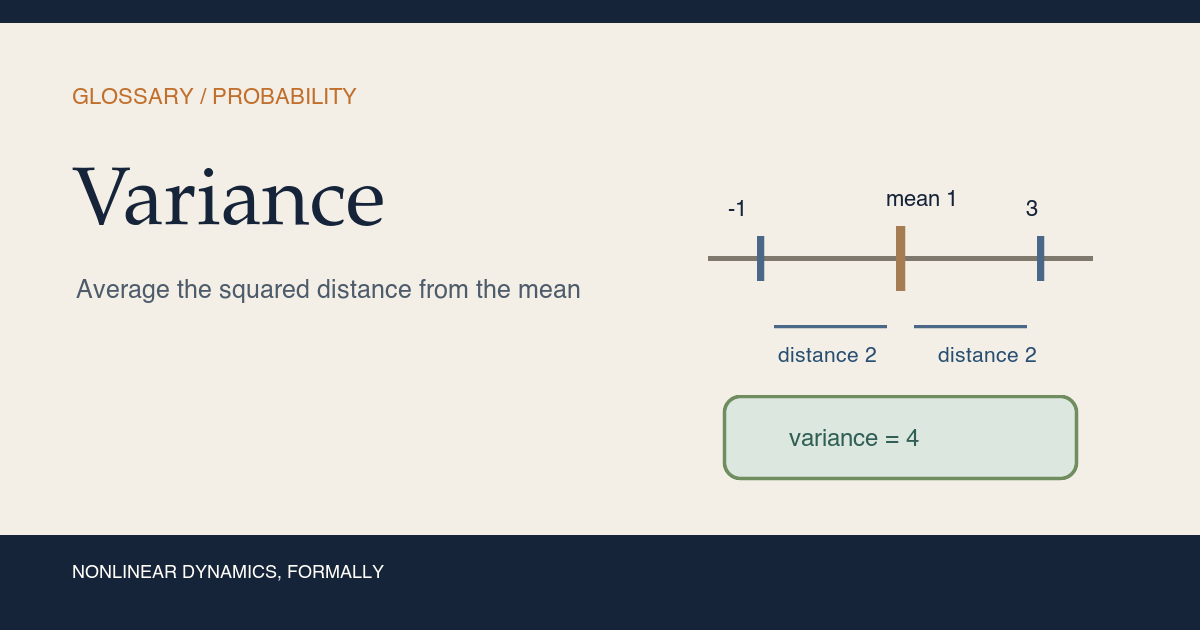
Variance measures squared spread around a mean. If a real random variable \(X\) is defined under a probability measure \(\mathbb P\), has finite second moment, and has mean

then its variance is

The subtraction measures a deviation from the center. Squaring makes positive and negative deviations contribute equally and weights large deviations more heavily. The expectation averages those squared deviations according to the probability law of \(X\).

Work one example all the way through

Let \(X\) take the values \(-1\) and \(3\), each with probability \(1/2\). Its mean is

Both values lie two units from the mean:

Their squared deviations are both \(4\), so

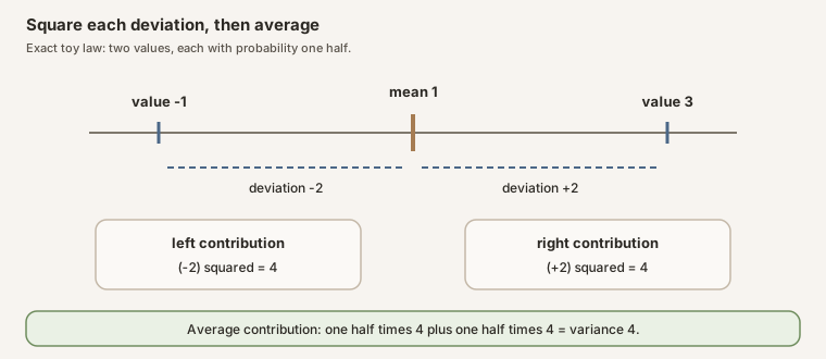
The standard deviation is the square root of variance, so this example has standard deviation \(2\). Variance has squared units. If \(X\) is measured in meters, then \(\operatorname{Var}(X)\) is measured in square meters, while its standard deviation returns to meters.

The rules that make variance useful

For a square-integrable real random variable and real constant \(c\):

because translation moves both \(X\) and its mean by the same amount. Scaling has a different effect:

This square is why a Gaussian law parameterized by variance \(v\) is built from a standard Gaussian by multiplying by \(\sqrt{v}\), not by \(v\).

For two square-integrable variables \(X\) and \(Y\),

where covariance records their joint linear co-movement. When \(X\) and \(Y\) are independent , their covariance vanishes under the usual integrability assumptions, so their variances add. The converse is false: zero covariance does not generally imply independence.

Zero variance and almost-sure constancy

If \(X\) is square-integrable under a probability measure, then

The phrase “almost surely” matters. A random variable may differ from its mean on a set of probability zero and still have zero variance. Zero variance does not force literal function equality at every outcome.

For the exact Gaussian law \(\gamma_{m,0}\), the same statement appears at the law level: \(\gamma_{m,0}=\delta_m\). The project theorem HasRealGaussianLaw.ae_eq_const_of_variance_zero turns that Dirac law into almost-everywhere equality with \(m\).

Population variance is not a finite-sample recipe

The definition above is population variance: an integral with respect to a probability law. Given observed data \(x_1,\ldots,x_n\), one can instead compute descriptive or inferential sample statistics. Two familiar formulas are

where \(\bar{x}\) is the sample mean. The second expression requires \(n\gt 1\). They answer different questions and use different denominators. Neither denominator belongs silently in the measure-theoretic definition of \(\operatorname{Var}_{\mathbb P}(X)\).

In Lean: write the variable and the measure explicitly

Var[X; P] = 4

For an almost-everywhere measurable \(X\), the integral formula appears as:

ProbabilityTheory.variance_eq_integral hX

Standalone tutorial

This first worksheet imports only Lean’s small Std library. It checks the arithmetic of the \(-1,3\) example without restoring Mathlib or building this repository. Create a scratch file named VarianceTiny.lean:

import Std

def square (z : Int) : Int := z * z

#eval [(-1 : Int), 3].map (fun x => square (x - 1))

example :
    square ((-1 : Int) - 1) + square (3 - 1) = 2 * 4 := by
  decide

Then type:

elan run leanprover/lean4:v4.32.0 lean VarianceTiny.lean

With the pinned Lean 4.32.0 toolchain, the evaluator prints [4, 4]. The theorem proves that the sum of the two squared deviations is \(2\cdot4\); dividing by the two equal probability weights gives variance \(4\). Change the claimed right-hand side to 2 * 5 and Lean should reject the file. That deliberate failure is the quickest way to feel the difference between evaluation and proof.

Full project check

On a clone with the repository’s pinned dependencies installed, a human can put this in a scratch Lean file:

import NonlinearDynamics.Random.GaussianPrimitives

open MeasureTheory ProbabilityTheory
open scoped ProbabilityTheory

#check ProbabilityTheory.evariance
#check ProbabilityTheory.variance
#check ProbabilityTheory.variance_eq_integral
#check ProbabilityTheory.variance_const_mul
#check ProbabilityTheory.IndepFun.variance_add
#check NonlinearDynamics.Random.HasRealGaussianLaw.variance_eq
#check NonlinearDynamics.Random.HasRealGaussianLaw.ae_eq_const_of_variance_zero

The first two checks expose both codomains. The next three inspect the integral, scaling, and independent-sum rules. The final two are project theorems: an exact Gaussian has the stated variance, and zero Gaussian variance yields equality with the mean almost everywhere.

cd formalization
lake env lean -DwarningAsError=true NonlinearDynamics/Random/GaussianPrimitives.lean

Why the pinned real-valued notation needs care

Mathlib 4.32.0 defines two related quantities:

• evariance X P : ℝ≥0∞ is an extended nonnegative real and can take the value infinity;
• variance X P : ℝ, written Var[X; P], applies ENNReal.toReal to extended variance.

The real-valued operation is total. In Mathlib it returns zero when the extended variance is infinite. Therefore a raw equality Var[X; P] = 0 must not be interpreted as almost-sure constancy unless a finite second-moment hypothesis rules out the infinite case.

For measurable \(X\), Mathlib’s finite-variance identity is exposed as variance_eq_integral:

#check ProbabilityTheory.variance_eq_integral
#check ProbabilityTheory.variance_const_mul
#check ProbabilityTheory.IndepFun.variance_add

The project’s exact Gaussian predicate avoids the totalization trap because a Gaussian variable belongs to every finite \(L^p\) space. Its theorem HasRealGaussianLaw.variance_eq states

Var[X; P] = (v : ℝ)

for the explicit nonnegative-real parameter v : ℝ≥0.

Edge cases and nonclaims

• Variance requires a measure. A bare function has no variance until a measure on its domain is fixed.
• Variance may be infinite. The extended quantity is the appropriate target before square integrability has been proved.
• A finite variance does not imply a Gaussian law. Many non-Gaussian laws have the same mean and variance.
• Variance summarizes one aspect of spread. It does not determine tail shape, skewness, multimodality, or dependence with other variables.
• Variance zero means almost-sure constancy under the stated hypotheses, not pointwise constancy on every element of the sample space.
• For a complex variable, one must say whether “variance” means \(\mathbb E|Z-\mathbb E Z|^2\), a covariance matrix of real and imaginary parts, a pseudocovariance, or another convention.

Where to continue

The Gaussian distribution uses variance as its exact spread parameter. The normalization convention page explains why scaling choices must be written down before real coordinates are assembled into a complex variable or matrix. The Cartesian complex Gaussian law keeps both component variances explicit, while Complex Gaussian Coordinates and Geometry derives their sum, difference, support geometry, and symmetry boundary. The earlier Gaussian Laws, Independence, and Normalization builds the real finite-product foundation.

References

Mathlib contributors. Variance of random variables, Mathlib 4 documentation. This official API reference documents evariance, the totalized real variance, scaling, and variance addition under independence.

Mathlib contributors. Gaussian distributions over the reals, Mathlib 4 documentation. The results variance_id_gaussianReal and memLp_id_gaussianReal connect the parameter \(v\) to finite variance and all finite moments.

National Institute of Standards and Technology. What do we mean by normal data?, Engineering Statistics Handbook. This official reference distinguishes a normal law’s variance from its standard deviation.

The local formalization uses the exact Mathlib 4.32.0 dependency pinned at commit 81a5d257.